Como criar uma lista suspensa com várias caixas de seleção no Excel?
As listas suspensas tradicionais no Excel limitam os usuários a seleções únicas. Para superar essa limitação e permitir múltiplas seleções, exploraremos dois métodos práticos para criar listas suspensas com várias caixas de seleção.
Use a Caixa de Listagem para criar uma lista suspensa com várias caixas de seleção
A: Crie uma caixa de listagem com dados de origem
B: Nomeie a célula onde você localizará os itens selecionados
C: Insira uma forma para ajudar a exibir os itens selecionados
Crie facilmente uma lista suspensa com caixas de seleção usando uma ferramenta incrível
Mais tutoriais para lista suspensa...
Use a Caixa de Listagem para criar uma lista suspensa com várias caixas de seleção
Como mostrado na captura de tela abaixo, todos os nomes no intervalo A2:A11 na planilha atual servirão como dados de origem para a caixa de listagem localizada na célula C4. Clicar nesta caixa expande a lista de itens que você pode selecionar, e os itens selecionados serão exibidos na célula E4. Para alcançar isso, siga estas etapas:

A. Crie uma caixa de listagem com dados de origem
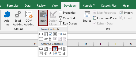
1. Clique em Desenvolvedor > Inserir > Caixa de Listagem (Controle ActiveX). Veja a captura de tela:
2. Desenhe uma caixa de listagem na planilha atual, clique com o botão direito nela e selecione Propriedades no menu de contexto.

3. Na caixa de diálogo Propriedades, você precisa configurar conforme segue.
- 3.1 Na caixa ListFillRange, insira o intervalo de origem que você deseja exibir na lista (aqui eu insiro o intervalo A2:A11);
- 3.2 Na caixa ListStyle, selecione 1 - fmListStyleOption;
- 3.3 Na caixa MultiSelect, selecione 1 – fmMultiSelectMulti;
- 3.4 Feche a caixa de diálogo Propriedades. Veja a captura de tela:


B: Nomeie a célula onde você localizará os itens selecionados
Se você precisar exibir todos os itens selecionados em uma célula específica, como E4, faça o seguinte.
1. Selecione a célula E4, insira ListBoxOutput na Caixa de Nome e pressione a tecla Enter.

C. Insira uma forma para ajudar a exibir os itens selecionados
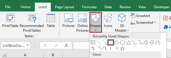
1. Clique em Inserir > Formas > Retângulo. Veja a captura de tela:
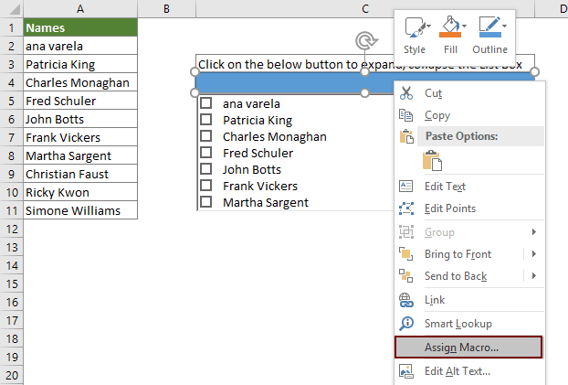
2. Desenhe um retângulo na sua planilha (aqui desenho o retângulo na célula C4). Em seguida, clique com o botão direito no retângulo e selecione Atribuir Macro no menu de contexto.
3. Na caixa de diálogo Atribuir Macro, clique no botão Novo.

4. Na janela Microsoft Visual Basic for Applications aberta, substitua o código original na janela Módulo pelo seguinte código VBA.
Código VBA: Criar uma lista com várias caixas de seleção
Sub Rectangle1_Click()
'Updated by Extendoffice 20200730
Dim xSelShp As Shape, xSelLst As Variant, I, J As Integer
Dim xV As String
Set xSelShp = ActiveSheet.Shapes(Application.Caller)
Set xLstBox = ActiveSheet.ListBox1
If xLstBox.Visible = False Then
    xLstBox.Visible = True
    xSelShp.TextFrame2.TextRange.Characters.Text = "Pickup Options"
    xStr = ""
    xStr = Range("ListBoxOutput").Value

    If xStr <> "" Then
         xArr = Split(xStr, ";")
    For I = xLstBox.ListCount - 1 To 0 Step -1
        xV = xLstBox.List(I)
        For J = 0 To UBound(xArr)
            If xArr(J) = xV Then
              xLstBox.Selected(I) = True
              Exit For
            End If
        Next
    Next I
    End If
Else
    xLstBox.Visible = False
    xSelShp.TextFrame2.TextRange.Characters.Text = "Select Options"
    For I = xLstBox.ListCount - 1 To 0 Step -1
        If xLstBox.Selected(I) = True Then
        xSelLst = xLstBox.List(I) & ";" & xSelLst
        End If
    Next I
    If xSelLst <> "" Then
        Range("ListBoxOutput") = Mid(xSelLst, 1, Len(xSelLst) - 1)
    Else
        Range("ListBoxOutput") = ""
    End If
End If
End Sub
Nota: No código, Rectangle1 é o nome da forma; ListBox1 é o nome da caixa de listagem; Selecionar Opções e Coletar Opções são os textos exibidos da forma; e ListBoxOutput é o nome do intervalo da célula de saída. Você pode alterá-los conforme necessário.
5. Pressione simultaneamente as teclas Alt + Q para fechar a janela Microsoft Visual Basic for Applications.
6. Clicando no botão retangular, a caixa de listagem será recolhida ou expandida. Quando a caixa de listagem estiver expandida, selecione os itens desejados marcando-os. Depois, clique novamente no retângulo para exibir todos os itens selecionados na célula E4. Veja a demonstração abaixo:
7. E então salve a pasta de trabalho como uma Pasta de Trabalho Habilitada para Macro do Excel para reutilizar o código no futuro.
Criar lista suspensa com caixas de seleção com uma ferramenta incrível
Cansado da codificação VBA complexa? O Kutools para Excel facilita a criação de listas suspensas com caixas de seleção para seleção múltipla perfeita. Perfeito para pesquisas, filtragem de dados ou formulários dinâmicos, esta ferramenta amigável simplifica seu fluxo de trabalho e economiza tempo.
1. Abra a planilha onde você configurou a validação de dados da lista suspensa, clique em Kutools > Lista Suspensa > Habilitar Lista Suspensa Avançada. Em seguida, clique em Lista Suspensa com Caixas de Seleção novamente na Lista Suspensa. Veja a captura de tela:
 |  |
2. Na caixa de diálogo Adicionar Caixas de Seleção à Lista Suspensa, configure conforme segue.
- 2.1) Selecione as células contendo a lista suspensa;
- 2.2) Na caixa Separador, insira um delimitador que você usará para separar os vários itens;
- 2.3) Marque a opção Ativar pesquisa conforme necessário. (Se marcar esta opção, poderá fazer uma busca posteriormente na lista suspensa.)
- 2.4) Clique no botão OK.


A partir de agora, quando você clicar na célula com a lista suspensa, uma caixa de listagem aparecerá, selecione os itens marcando as caixas de seleção para exibi-los na célula, conforme mostrado na demonstração abaixo.
Para mais detalhes sobre este recurso, visite este tutorial.
Kutools para Excel - Potencialize o Excel com mais de 300 ferramentas essenciais. Aproveite recursos de IA permanentemente gratuitos! Obtenha Agora
Este artigo fornece dois métodos para ajudá-lo a criar facilmente listas suspensas com caixas de seleção no Excel. Você pode escolher aquele que preferir. Se você estiver interessado em explorar mais dicas e truques do Excel, nosso site oferece milhares de tutoriais.
Artigos relacionados:
Autocompletar ao digitar na lista suspensa do Excel
Se você tiver uma lista suspensa de validação de dados com muitos valores, precisará rolar pela lista apenas para encontrar o valor adequado ou digitar a palavra inteira diretamente na caixa de listagem. Se houver um método que permita autocompletar ao digitar a primeira letra na lista suspensa, tudo ficará mais fácil. Este tutorial fornece o método para resolver o problema.
Criar lista suspensa a partir de outra pasta de trabalho no Excel
É muito fácil criar uma lista suspensa de validação de dados entre planilhas dentro de uma pasta de trabalho. Mas se os dados da lista que você precisa para a validação estiverem em outra pasta de trabalho, o que você faria? Neste tutorial, você aprenderá em detalhes como criar uma lista suspensa a partir de outra pasta de trabalho no Excel.
Criar uma lista suspensa pesquisável no Excel
Para uma lista suspensa com inúmeros valores, encontrar o valor adequado não é uma tarefa fácil. Anteriormente, introduzimos um método de autocompletar a lista suspensa ao inserir a primeira letra na caixa suspensa. Além da função de autocompletar, você também pode tornar a lista suspensa pesquisável para aumentar a eficiência no trabalho ao encontrar valores adequados na lista suspensa. Para tornar a lista suspensa pesquisável, experimente o método neste tutorial.
Preencher automaticamente outras células ao selecionar valores na lista suspensa do Excel
Digamos que você tenha criado uma lista suspensa com base nos valores no intervalo de células B8:B14. Ao selecionar qualquer valor na lista suspensa, você quer que os valores correspondentes no intervalo de células C8:C14 sejam automaticamente preenchidos em uma célula selecionada. Para resolver o problema, os métodos deste tutorial ajudarão.
Melhores Ferramentas de Produtividade para Office
Impulsione suas habilidades no Excel com Kutools para Excel e experimente uma eficiência incomparável. Kutools para Excel oferece mais de300 recursos avançados para aumentar a produtividade e economizar tempo. Clique aqui para acessar o recurso que você mais precisa...
Office Tab traz interface com abas para o Office e facilita muito seu trabalho
- Habilite edição e leitura por abas no Word, Excel, PowerPoint, Publisher, Access, Visio e Project.
- Abra e crie múltiplos documentos em novas abas de uma mesma janela, em vez de em novas janelas.
- Aumente sua produtividade em50% e economize centenas de cliques todos os dias!
Todos os complementos Kutools. Um instalador
O pacote Kutools for Office reúne complementos para Excel, Word, Outlook & PowerPoint, além do Office Tab Pro, sendo ideal para equipes que trabalham em vários aplicativos do Office.
- Pacote tudo-em-um — complementos para Excel, Word, Outlook & PowerPoint + Office Tab Pro
- Um instalador, uma licença — configuração em minutos (pronto para MSI)
- Trabalhe melhor em conjunto — produtividade otimizada entre os aplicativos do Office
- Avaliação completa por30 dias — sem registro e sem cartão de crédito
- Melhor custo-benefício — economize comparado à compra individual de add-ins