Ir para o conteúdo principal

Como encontrar a enésima célula não em branco no Excel?

Autor: Xiao Yang Última modificação: 2020-07-03

Como você poderia encontrar e retornar o enésimo valor de célula não em branco de uma coluna ou linha no Excel? Neste artigo, irei falar sobre algumas fórmulas úteis para você resolver esta tarefa.

Encontre e retorne o enésimo valor de célula não em branco de uma coluna com fórmula

Encontre e retorne o enésimo valor de célula não em branco de uma linha com fórmula


seta azul bolha direita Encontre e retorne o enésimo valor de célula não em branco de uma coluna com fórmula

Por exemplo, eu tenho uma coluna de dados conforme a captura de tela a seguir mostrada, agora, vou obter o terceiro valor de célula não em branco desta lista.

doc encontrar enésimo não em branco 1

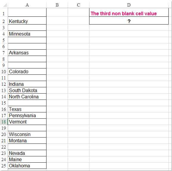
Insira esta fórmula: =INDEX($A$1:$A$25,SMALL(ROW($A$1:$A$25)+(100*($A$1:$A$25="")), 3))&"" em uma célula em branco onde você deseja produzir o resultado, D2, por exemplo, e pressione Ctrl + Shift + Enter juntas para obter o resultado correto, veja a captura de tela:

doc encontrar enésimo não em branco 2

Note: Na fórmula acima, A1: A25 é a lista de dados que você deseja usar e o número 3 indica o terceiro valor de célula não em branco que você deseja retornar, se você deseja obter a segunda célula não em branco, você só precisa alterar o número 3 para 2 conforme necessário.


seta azul bolha direita Encontre e retorne o enésimo valor de célula não em branco de uma linha com fórmula

Se você quiser encontrar e retornar o enésimo valor de célula não em branco em uma linha, a seguinte fórmula pode ajudá-lo, faça o seguinte:

Insira esta fórmula: =INDEX($A$1:$M$1,SMALL(IF($A$1:$M$1<>"",COLUMN($A$1:$M$1)-COLUMN($A$1)+1),4)) em uma célula em branco onde você deseja localizar o resultado e pressione Ctrl + Shift + Enter juntas para obter o resultado, consulte a captura de tela:

doc encontrar enésimo não em branco 3

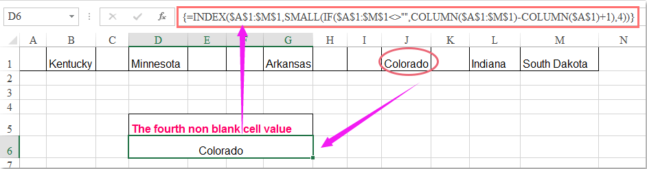
Observação: Na fórmula acima, A1: M1 são os valores da linha que você deseja usar e o número 4 é o quarto valor de célula não em branco que você deseja retornar, se você quiser obter a segunda célula não em branco, você só precisa alterar o número 4 para 2 conforme necessário.

Melhores ferramentas de produtividade de escritório

🤖 Assistente de IA do Kutools: Revolucionar a análise de dados com base em: Execução Inteligente   |  Gerar Código  |  Crie fórmulas personalizadas  |  Analise dados e gere gráficos  |  Invocar funções do Kutools...
Recursos mais comuns: Encontre, destaque ou identifique duplicatas   |  Excluir linhas em branco   |  Combine colunas ou células sem perder dados   |   Rodada sem Fórmula ...
Super pesquisa: VLookup de múltiplos critérios    VLookup de múltiplos valores  |   VLookup em várias planilhas   |   Pesquisa Difusa ....
Lista suspensa avançada: Crie rapidamente uma lista suspensa   |  Lista suspensa de dependentes   |  Lista suspensa de seleção múltipla ....
Gerenciador de colunas: Adicione um número específico de colunas  |  Mover colunas  |  Alternar status de visibilidade de colunas ocultas  |  Compare intervalos e colunas ...
Recursos em destaque: Foco da Grade   |  Vista de Design   |   Grande Barra de Fórmula    Gerenciador de pastas de trabalho e planilhas   |  Biblioteca (Auto texto)   |  Data Picker   |  Combinar planilhas   |  Criptografar/Descriptografar Células    Enviar e-mails por lista   |  Super Filtro   |   Filtro Especial (filtro negrito/itálico/tachado...) ...
15 principais conjuntos de ferramentas12 Texto Ferramentas (Adicionar texto, Remover Personagens, ...)   |   50+ de cores Tipos (Gráfico de Gantt, ...)   |   Mais de 40 práticos Fórmulas (Calcule a idade com base no aniversário, ...)   |   19 Inclusão Ferramentas (Insira o código QR, Inserir imagem do caminho, ...)   |   12 Conversão Ferramentas (Números para Palavras, Conversão de moedas, ...)   |   7 Unir e dividir Ferramentas (Combinar linhas avançadas, Dividir células, ...)   |   ... e mais

Aprimore suas habilidades de Excel com o Kutools para Excel e experimente uma eficiência como nunca antes. Kutools para Excel oferece mais de 300 recursos avançados para aumentar a produtividade e economizar tempo.  Clique aqui para obter o recurso que você mais precisa...

Descrição


Office Tab traz interface com guias para o Office e torna seu trabalho muito mais fácil

  • Habilite a edição e leitura com guias em Word, Excel, PowerPoint, Publisher, Access, Visio e Project.
  • Abra e crie vários documentos em novas guias da mesma janela, em vez de em novas janelas.
  • Aumenta sua produtividade em 50% e reduz centenas de cliques do mouse para você todos os dias!
Comments (10)
No ratings yet. Be the first to rate!
This comment was minimized by the moderator on the site
CIAO STO CERCANDO DI APPLICARE LA TUA FORMULA MA NON MI FUNZIONA, DOVE STO SBAGLIANDO?
=INDICE($K$37:$K$88;MIN(RIGHE($K$37:$K$88)+RIGHE(100*($K$37:$K$88=""));6))&""
DEVO VISUALIZZARE L'ENNESIMA RIGA DIVERSA DA VUOTO

GRAzie
This comment was minimized by the moderator on the site
=INDICE($K$37:$K$88;MIN(RIGHE($K$37:$K$88)+(100*($K$37:$K$88=""));6))&""
This comment was minimized by the moderator on the site
I'm running this formula on a ~400 row sheet with around 20 blanks mixed throughout the data, and it's working perfectly EXCEPT when I fill the series down, it sometimes duplicates a row for some reason. For example, it seems to think a value is somehow simultaneously the 331st non-blank and the 332nd.

Things I've noticed:
-Duplications always happen in pairs (ex. 331 and 332 are duplicates, 333 and 334 will also be), then it goes back to normal for a while.
-Raw data also has blanks in pairs, but not corresponding to the duplicates
-No duplications occur in the first 94 rows, but they happen every 33-35 rows after that
-Does not appear to be linked to the value in the cell being duplicated
-I have entered as an array and as a standard formula, no difference in function

For reference, here's my actual formula:

=INDEX('PO Raw Data'!CR:CR,SMALL(ROW('PO Raw Data'!CR:CR)+(100*('PO Raw Data'!CR:CR="")),$W2)&"")

Note $W2 refers to a helper column and counts up as the data set is filled down, but only because I couldn't get it to count up when I just used a number instead of cell reference.
When I've replaced that cell reference (ex. $W2) with the appropriate number, same result.


Any thoughts on what I can do to fix that?
This comment was minimized by the moderator on the site
very helpful,
although when I return the nth non blank cell in a column set to DATE, the returned value appears as number(general number).formatting the cell into DATE also doesn't change the result. could you please give me a hand!
thanks a lot
This comment was minimized by the moderator on the site
Hello, Shirazi,
Sorry, maybe there is no direct formula for you to get the date format.

If someone else has the solution, please comment here.
This comment was minimized by the moderator on the site
Hi everyone!


Could you also help me return the row number of the second, third non-blank cell?


Please help me.
This comment was minimized by the moderator on the site
Hello, John,
the following formula can help you to get all the row numbers of the non-blank cells, please try it, thank you!
=IFERROR(ROW(INDEX($A$1:$A$12,SMALL(INDEX(NOT(ISBLANK($A$1:$A$12))*ROW($A$1:$A$12),0),COUNTBLANK($A$1:$A$12)+ROW(A1)))),"")
This comment was minimized by the moderator on the site
Hey everyone,

I have a table with numerous columns and rows. The rows have range names, and a description/location at the beginning of the row range with its own range, example "Building No.s". There are multiple Row Ranges/ Buildings. There are headers at the top of each columns for specific "Building Assembly Types". The table content is numeric quantities for each type "Building Assembly Type" for each specific "Building" description/location. There could be as many as (100) "Building Assembly Types" column headers but I will limit the assemblies to (10) per row range, so there will be numerous blank cells in each "Building No." range.

I have other summary tables set up for each "Building" that I want to pull the non-blank cells quantities to, along with the corresponding header "Assembly Type" for each "Building" with a (10) max "Assemblies" per page.

I can identify the non-blank cell quantities by use of the array formula above for rows. The problem I am having is identifying the header that corresponds to it.

Ultimately if I can identify the "Assembly" header, I can always index the "Quantities" once I have the header "Assembly" identified for each "Building". Then I would be able do a lookup for all the parts associated with each "Assembly" type for that "Building" from my Assembly parts database and multiply it times the "Quantity" of each assembly type.

Hopefully this makes since and someone can help.
This comment was minimized by the moderator on the site
Hello, I am looking for the third blank row in a column and I copied your formula and just changed the range from $A$1:$A:$25 to my range $D$306:$D$354. But when I change the range I get #REF! as my answer. I already converted to an array, control-shift-enter. Now the cell range I am referencing has formulas in them, so could that be why I am getting #REF. Your formula: =INDEX($A$1:$A$25,SMALL(ROW($A$1:$A$25)+(100*($A$1:$A$25="")), 3))&"" My formula: =INDEX($D$306:$D$354,SMALL(ROW($D$306:$D$354)+(1*($D$306:$D$354="")), 2))&"" Thanks, Noel
This comment was minimized by the moderator on the site
you have put the 1 instead of 100 therefore answered was wrong. please use below formula

INDEX($D$306:$D$354,SMALL(ROW($D$306:$D$354)+(100*($D$306:$D$354="")), 3))&"" than ctrl + shift+enter
There are no comments posted here yet
Please leave your comments in English
Posting as Guest
×
Rate this post:
0   Characters
Suggested Locations