Retornar vários valores correspondentes com base em vários critérios no Excel (Guia completa)
Os usuários do Excel frequentemente encontram cenários onde é necessário extrair vários valores que satisfaçam vários critérios simultaneamente e apresentar todos os resultados correspondentes em uma coluna, linha ou consolidados em uma única célula. Este guia explora métodos para todas as versões do Excel, bem como a nova função FILTER disponível no Excel 365 e 2021.
Retornar vários valores correspondentes com base em múltiplos critérios em uma única célula
No Excel, extrair vários valores correspondentes com base em múltiplos critérios dentro de uma única célula é um desafio comum. Aqui estão dois métodos eficientes.
Método 1: Usando a função Textjoin (Excel 365 / 2021, 2019)
Para obter todos os valores correspondentes em uma única célula com delimitadores, a função TEXTJOIN pode ajudá-lo.
Digite ou copie a seguinte fórmula em uma célula em branco, depois pressione a tecla Enter (Excel 2021 e Excel 365) ou Ctrl + Shift + Enter no Excel 2019 para obter o resultado:
=TEXTJOIN(", ", TRUE, IF(($A$2:$A$18=E2)*($B$2:$B$18=F2), $C$2:$C$18, ""))
- ($A$2:$A$21=E2)*($B$2:$B$21=F2) verifica se cada linha atende ambas as condições: “Vendedor igual a E2” e “Mês igual a F2”. Se ambas as condições forem atendidas, o resultado será 1; caso contrário, será 0. O asterisco * significa que ambas as condições devem ser verdadeiras.
- SE(..., $C$2:$C$21, "") retorna o nome do produto se a linha corresponder; caso contrário, retorna um espaço em branco.
- TEXTJOIN(", ", VERDADEIRO, ...) combina todos os nomes de produtos não vazios em uma célula, separados por ", ".
Método 2: Usando Kutools para Excel
Kutools para Excel oferece uma solução poderosa e simples, permitindo que você recupere rapidamente e combine várias correspondências em uma única célula com base em múltiplos critérios sem fórmulas complexas.
Após instalar o Kutools para Excel, proceda da seguinte forma:
- Selecione o intervalo de dados que deseja usar para obter todos os valores correspondentes com base nos critérios.
- Em seguida, clique em Kutools > Mesclar e Dividir > Mesclar Linhas Avançado, veja a captura de tela:

- Na caixa de diálogo Mesclar Linhas Avançadas, configure as seguintes opções:
- Escolha os cabeçalhos das colunas que contêm seus critérios de correspondência (por exemplo, Vendedor e Mês). Para cada coluna selecionada, clique em Chave Primária para defini-las como suas condições de pesquisa.
- Clique no cabeçalho da coluna onde deseja os resultados combinados (por exemplo, Produto). Na seção Combinar, selecione seu delimitador preferido (por exemplo, vírgula, espaço ou separador personalizado).
- Por fim, clique no botão OK.


Resultado: Kutools irá instantaneamente mesclar todos os valores correspondentes em uma única célula para cada combinação exclusiva de critérios.

Retornar vários valores correspondentes com base em múltiplos critérios em uma coluna
Quando você precisa extrair e exibir vários registros correspondentes de um conjunto de dados com base em várias condições, retornando os resultados em formato vertical de coluna, o Excel oferece várias soluções poderosas.
Método 1: Usando uma fórmula de matriz (para todas as versões)
Você pode usar a seguinte fórmula de matriz para retornar resultados verticalmente em uma coluna:
1. Copie ou insira a seguinte fórmula em uma célula em branco:
=IFERROR(INDEX($C$2:$C$18, SMALL(IF(($A$2:$A$18=$E$2)*($B$2:$B$18=$F$2), ROW($C$2:$C$18)-ROW($C$2)+1), ROW(1:1))), "")2. Pressione Ctrl + Shift + Enter para obter o primeiro resultado correspondente, e então selecione a primeira célula da fórmula e arraste a alça de preenchimento para baixo até que apareça uma célula em branco; agora, todos os valores correspondentes são retornados conforme mostrado na captura de tela abaixo:

- $A$2:$A$18=$E$2: Verifica se o Vendedor corresponde ao valor na célula E2.
- $B$2:$B$18=$F$2: Verifica se o Mês corresponde ao valor na célula F2.
- * é um operador lógico E (ambas as condições devem ser verdadeiras).
- LIN($C$2:$C$18)-LIN($C$2)+1: Gera um número relativo de linha para cada produto.
- MENOR(..., LIN(1:1)): Busca o n-ésimo menor número de linha correspondente (à medida que a fórmula é arrastada para baixo).
- ÍNDICE(...): Retorna o produto da linha correspondente.
- SEERRO(..., ""): Retorna uma célula em branco se não houver mais correspondências.
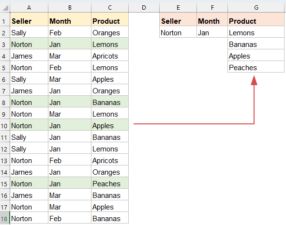
Método 2: Usando a função Filter (Excel 365 / 2021)
Se você estiver usando o Excel 365 ou o Excel 2021, a função FILTER é uma excelente escolha para retornar múltiplos resultados com base em vários critérios, graças à sua simplicidade, clareza e capacidade de derramar resultados dinamicamente sem fórmulas de matriz complexas.
Copie ou insira a fórmula abaixo em uma célula em branco, depois pressione a tecla Enter; todos os registros correspondentes serão retornados com base nos múltiplos critérios.
=FILTER(C2:C18, (A2:A18=E2)*(B2:B18=F2), "No match")
- FILTRO(...) retorna todos os valores de C2:C18 onde ambas as condições são atendidas.
- (A2:A18=E2)*(B2:B18=F2): Array lógico que verifica correspondência de vendedor e mês.
- "Nenhuma correspondência": Mensagem opcional se nenhum valor for encontrado.
Retornar vários valores correspondentes com base em múltiplos critérios em uma linha
Os usuários do Excel muitas vezes precisam extrair vários valores de um conjunto de dados que atendam a várias condições e exibi-los horizontalmente (em uma linha). Isso é útil para criar relatórios dinâmicos, painéis de controle ou tabelas de resumo onde o espaço vertical é limitado. Nesta seção, exploraremos dois métodos poderosos.
Método 1: Usando uma fórmula de matriz (para todas as versões)
As fórmulas de matriz tradicionais permitem extrair vários valores correspondentes usando funções como ÍNDICE, MENOR, SE e COLUNA. Ao contrário da extração vertical (baseada em coluna), ajustamos a fórmula para retornar resultados em uma linha.
1. Copie ou insira a fórmula abaixo em uma célula em branco:
=IFERROR(INDEX($C$2:$C$18, SMALL(IF(($A$2:$A$18=$E$2)*($B$2:$B$18=$F$2), ROW($C$2:$C$18)-ROW($C$2)+1), COLUMN(A1))), "")2. Pressione Ctrl + Shift + Enter para obter o primeiro resultado correspondente, e então selecione a primeira célula da fórmula e arraste a fórmula para a direita através das colunas para recuperar todos os resultados.

- $A$2:$A$18=$E$2: Verifica se o Vendedor corresponde.
- $B$2:$B$18=$F$2: Verifica se o Mês corresponde.
- *: Lógica E — ambas as condições devem ser verdadeiras.
- LIN($C$2:$C$18)-LIN($C$2)+1: Cria números relativos de linha.
- COL(A1): Ajusta qual correspondência retornar, dependendo de quão longe a fórmula foi arrastada para a direita.
- SEERRO(...): Evita erros quando as correspondências se esgotarem.
Método 2: Usando a função Filter (Excel 365 / 2021)
Copie ou insira a fórmula abaixo em uma célula em branco, depois pressione a tecla Enter; todos os valores correspondentes serão extraídos e localizados em uma linha. Veja a captura de tela:
=TRANSPOSE(FILTER(C2:C18, (A2:A18=E2)*(B2:B18=F2), "No match"))
- FILTRO(...): Recupera valores correspondentes da coluna C com base nas duas condições.
- (A2:A18=E2)*(B2:B18=F2): Ambas as condições devem ser verdadeiras.
- TRANSPOR(...): Converte a matriz vertical retornada pelo FILTRO em uma matriz horizontal.
🔚 Conclusão
Recuperar vários valores correspondentes com base em múltiplos critérios no Excel pode ser realizado de várias maneiras, dependendo de como você deseja exibir os resultados — seja em uma coluna, linha ou dentro de uma única célula.
- Para usuários com Excel 365 ou Excel 2021, a função FILTER oferece uma solução moderna, dinâmica e elegante que minimiza a complexidade.
- Para aqueles que usam versões mais antigas, as fórmulas de matriz permanecem ferramentas poderosas, embora exijam um pouco mais de configuração e cuidado.
- Além disso, se você quiser consolidar resultados em uma única célula ou preferir uma solução sem código, a função TEXTJOIN ou ferramentas de terceiros como Kutools para Excel podem simplificar significativamente o processo.
Escolha o método que melhor se adapta à sua versão do Excel e ao layout preferido, e você estará bem equipado para lidar com buscas multicritério de forma eficiente e precisa. Se você está interessado em explorar mais dicas e truques do Excel, nosso site oferece milhares de tutoriais para ajudá-lo a dominar o Excel.
Mais artigos relacionados:
- Retornar Múltiplos Valores de Pesquisa Em Uma Célula Separada Por Vírgulas
- No Excel, podemos aplicar a função PROCV para retornar o primeiro valor correspondente de uma tabela, mas às vezes precisamos extrair todos os valores correspondentes e separá-los por um delimitador específico, como vírgula, traço, etc., em uma única célula conforme mostrado na captura de tela a seguir. Como obter e retornar múltiplos valores de pesquisa em uma célula separada por vírgulas no Excel?
- Procurar e Retornar Múltiplos Valores Correspondentes Simultaneamente No Google Sheets
- A função PROCV normal no Google Sheets pode ajudá-lo a encontrar e retornar o primeiro valor correspondente com base em dados fornecidos. Mas, às vezes, você pode precisar procurar e retornar todos os valores correspondentes conforme mostrado na captura de tela a seguir. Você tem alguma boa e fácil maneira de resolver essa tarefa no Google Sheets?
- Procurar e Retornar Múltiplos Valores Da Lista Suspensa
- No Excel, como você faria para procurar e retornar múltiplos valores correspondentes de uma lista suspensa, o que significa que, quando você escolher um item da lista suspensa, todos os seus valores relativos serão exibidos de uma vez, conforme mostrado na captura de tela a seguir. Este artigo apresentará a solução passo a passo.
- Procurar e Retornar Múltiplos Valores Verticalmente No Excel
- Normalmente, você pode usar a função PROCV para obter o primeiro valor correspondente, mas, às vezes, você quer retornar todos os registros correspondentes com base em um critério específico. Este artigo falará sobre como procurar e retornar todos os valores correspondentes verticalmente, horizontalmente ou em uma única célula.
- Procurar e Retornar Dados Correspondentes Entre Dois Valores No Excel
- No Excel, podemos aplicar a função PROCV normal para obter o valor correspondente com base em dados fornecidos. Mas, às vezes, queremos procurar e retornar o valor correspondente entre dois valores, conforme mostrado na captura de tela a seguir. Como você lidaria com essa tarefa no Excel?
Melhores Ferramentas de Produtividade para Office
Impulsione suas habilidades no Excel com Kutools para Excel e experimente uma eficiência incomparável. Kutools para Excel oferece mais de300 recursos avançados para aumentar a produtividade e economizar tempo. Clique aqui para acessar o recurso que você mais precisa...
Office Tab traz interface com abas para o Office e facilita muito seu trabalho
- Habilite edição e leitura por abas no Word, Excel, PowerPoint, Publisher, Access, Visio e Project.
- Abra e crie múltiplos documentos em novas abas de uma mesma janela, em vez de em novas janelas.
- Aumente sua produtividade em50% e economize centenas de cliques todos os dias!
Todos os complementos Kutools. Um instalador
O pacote Kutools for Office reúne complementos para Excel, Word, Outlook & PowerPoint, além do Office Tab Pro, sendo ideal para equipes que trabalham em vários aplicativos do Office.
- Pacote tudo-em-um — complementos para Excel, Word, Outlook & PowerPoint + Office Tab Pro
- Um instalador, uma licença — configuração em minutos (pronto para MSI)
- Trabalhe melhor em conjunto — produtividade otimizada entre os aplicativos do Office
- Avaliação completa por30 dias — sem registro e sem cartão de crédito
- Melhor custo-benefício — economize comparado à compra individual de add-ins