Como aplicar formatação condicional com base em outra planilha no Google Sheets?
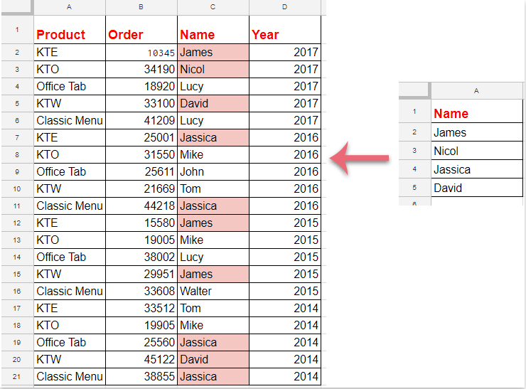
A formatação condicional é um recurso útil no Google Sheets que permite destacar automaticamente células com base em critérios específicos, facilitando a análise e visualização dos seus dados. Às vezes, em vez de destacar células de acordo com valores na mesma planilha, pode ser necessário basear suas regras de formatação em uma lista de referência ou critérios armazenados em uma planilha diferente. Por exemplo, você pode querer destacar células em uma planilha que também aparecem em uma lista mantida em outra planilha, como ilustrado na captura de tela abaixo. Esse tipo de tarefa é comum quando você está trabalhando com dados cruzados, como comparar vendas atuais com uma lista mestre de produtos ou verificar entradas duplicadas contra outra fonte de dados. No entanto, configurar esse tipo de formatação condicional no Google Sheets — especialmente ao fazer referência a dados de diferentes planilhas — pode ser confuso se você nunca o fez antes. O guia abaixo mostrará, passo a passo, uma abordagem simples para realizar isso.
Formatação condicional para destacar células com base em uma lista de outra planilha no Google Sheets
Esse método permite configurar uma regra de formato condicional para destacar células na sua planilha ativa se elas aparecerem em uma lista específica de outra planilha. Esse tipo de formatação condicional entre planilhas é particularmente útil para monitoramento dinâmico de dados e manutenção da consistência entre conjuntos de dados relacionados.
Para completar esse processo, siga estas etapas detalhadas:
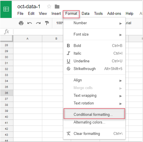
1. Abra sua planilha de destino, clique no menu Formatar na parte superior e selecione Formatação condicional. O painel Regras de formatação condicional será aberto no lado direito da sua tela.
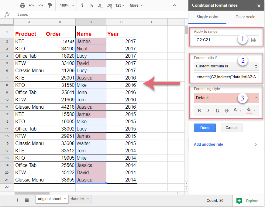
2. No painel Regras de formatação condicional, execute as seguintes ações:
(1.) Clique no ![]() botão ao lado do campo "Aplicar ao intervalo". Selecione o intervalo de células que deseja destacar. Por exemplo, se você quiser formatar todos os valores na coluna C a partir da linha 2 para baixo, selecione C2:C. Selecionar um intervalo apropriado garante que apenas as células pretendidas sejam avaliadas para formatação.
botão ao lado do campo "Aplicar ao intervalo". Selecione o intervalo de células que deseja destacar. Por exemplo, se você quiser formatar todos os valores na coluna C a partir da linha 2 para baixo, selecione C2:C. Selecionar um intervalo apropriado garante que apenas as células pretendidas sejam avaliadas para formatação.
(2.) No menu suspenso Formatar células se, escolha Fórmula personalizada é. Insira a seguinte fórmula na caixa fornecida: =match(C2,indirect("data list!A2:A"),0). Essa fórmula verifica se cada célula na coluna C corresponde a qualquer valor no intervalo A2:A da planilha "data list".
(3.) Em Estilo de formatação, selecione o estilo de formatação desejado, como preencher a célula com uma cor específica ou alterar o estilo da fonte. Você pode visualizar o estilo imediatamente na sua planilha antes de aplicá-lo.
Nota: Na fórmula acima, C2 refere-se à primeira célula no intervalo selecionado (ajuste se seus dados começarem em uma linha ou coluna diferente) e data list!A2:A refere-se ao nome da planilha (“data list”) e ao intervalo correspondente (A2:A) onde sua lista de outra planilha está armazenada. Certifique-se de que a referência de célula na fórmula corresponda à célula superior esquerda do seu intervalo selecionado; caso contrário, a formatação pode não ser aplicada corretamente. Se o intervalo da sua lista de dados for diferente, lembre-se de atualizá-lo na fórmula (por exemplo, “data list!B2:B”).
3. Uma vez configurada a regra, as células correspondentes no intervalo escolhido serão destacadas instantaneamente com base na lista da outra planilha. Revise a visualização e clique em Concluído na parte inferior do painel Regras de formatação condicional para aplicar e salvar sua formatação.
Dicas e solução de problemas:
- Verifique novamente erros tipográficos na sua fórmula, especialmente nos nomes das planilhas e nas referências de intervalo — referências incorretas são uma razão comum pela qual as regras falham.
- Se sua lista de dados contiver células em branco, a função
MATCHretornará um erro#N/Dpara valores não correspondentes, mas esse é um comportamento esperado e não afeta o destaque dos itens correspondentes. - Ao copiar a formatação para uma nova planilha ou ajustar intervalos, certifique-se de atualizar as referências de células na sua fórmula personalizada de acordo.
- A formatação é atualizada automaticamente se você adicionar ou remover itens da sua lista de referência posteriormente.
- A planilha e o intervalo referenciados na sua fórmula existem e estão escritos corretamente.
- A primeira célula na sua fórmula corresponde à primeira célula do intervalo selecionado.
- Todas as permissões necessárias para acesso entre planilhas dentro da sua planilha estão disponíveis — este método funciona dentro de um único arquivo do Google Sheets com várias planilhas, não entre arquivos diferentes.
Como alternativa, se a estrutura de dados ou requisitos forem mais complexos — por exemplo, se você precisar comparar várias colunas, permitir correspondências parciais ou realizar buscas mais avançadas — usar colunas auxiliares com fórmulas COUNTIF ou VLOOKUP, ou empregar o Google Apps Script (código JavaScript personalizado), também pode alcançar soluções flexíveis de formatação condicional.
Em resumo, configurar formatação condicional com base em outra planilha é altamente eficaz para verificação de listas, rastreamento de duplicatas e várias validações de dados entre planilhas — tudo dentro do Google Sheets. Sempre confirme suas entradas de fórmulas, intervalos de referência e regras de formatação para obter resultados suaves e precisos.

Desbloqueie a Magia do Excel com o Kutools AI
- Execução Inteligente: Realize operações de células, analise dados e crie gráficos — tudo impulsionado por comandos simples.
- Fórmulas Personalizadas: Gere fórmulas sob medida para otimizar seus fluxos de trabalho.
- Codificação VBA: Escreva e implemente código VBA sem esforço.
- Interpretação de Fórmulas: Compreenda fórmulas complexas com facilidade.
- Tradução de Texto: Supere barreiras linguísticas dentro de suas planilhas.
Melhores Ferramentas de Produtividade para Office
Impulsione suas habilidades no Excel com Kutools para Excel e experimente uma eficiência incomparável. Kutools para Excel oferece mais de300 recursos avançados para aumentar a produtividade e economizar tempo. Clique aqui para acessar o recurso que você mais precisa...
Office Tab traz interface com abas para o Office e facilita muito seu trabalho
- Habilite edição e leitura por abas no Word, Excel, PowerPoint, Publisher, Access, Visio e Project.
- Abra e crie múltiplos documentos em novas abas de uma mesma janela, em vez de em novas janelas.
- Aumente sua produtividade em50% e economize centenas de cliques todos os dias!
Todos os complementos Kutools. Um instalador
O pacote Kutools for Office reúne complementos para Excel, Word, Outlook & PowerPoint, além do Office Tab Pro, sendo ideal para equipes que trabalham em vários aplicativos do Office.
- Pacote tudo-em-um — complementos para Excel, Word, Outlook & PowerPoint + Office Tab Pro
- Um instalador, uma licença — configuração em minutos (pronto para MSI)
- Trabalhe melhor em conjunto — produtividade otimizada entre os aplicativos do Office
- Avaliação completa por30 dias — sem registro e sem cartão de crédito
- Melhor custo-benefício — economize comparado à compra individual de add-ins