Como criar uma lista suspensa dependente no Google Sheets?
Inserir uma lista suspensa normal no Google Sheets pode ser simples para você, mas às vezes, pode ser necessário criar uma lista suspensa dependente, onde a segunda lista depende da seleção na primeira lista. Como você poderia lidar com essa tarefa no Google Sheets?
Criar uma lista suspensa dependente no Google Sheets
Criar uma lista suspensa dependente no Google Sheets
Siga estas etapas para criar uma lista suspensa dependente no Google Sheets:
1. Primeiro, você deve inserir a lista suspensa básica, por favor, selecione uma célula onde deseja colocar a primeira lista suspensa e, em seguida, clique em Dados > Validação de dados, veja a captura de tela:

2. Na caixa que apareceu Validação de dados selecione Lista a partir de um intervalo a partir da lista suspensa ao lado da seção Critérios e, em seguida, clique no ![]() botão para selecionar os valores das células nos quais deseja criar a primeira lista suspensa com base, veja a captura de tela:
botão para selecionar os valores das células nos quais deseja criar a primeira lista suspensa com base, veja a captura de tela:

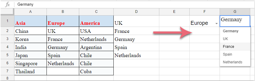
3. Em seguida, clique no botão Salvar, a primeira lista suspensa foi criada. Escolha um item da lista suspensa criada e, em seguida, insira esta fórmula: =arrayformula(se(F1=A1,A2:A7,se(F1=B1,B2:B6,se(F1=C1,C2:C7,"")))) em uma célula em branco adjacente às colunas de dados, depois pressione a tecla Enter; todos os valores correspondentes com base no item da primeira lista suspensa serão exibidos imediatamente, veja a captura de tela:
Observação: Na fórmula acima: F1 é a célula da primeira lista suspensa, A1, B1 e C1 são os itens da primeira lista suspensa, A2:A7, B2:B6 e C2:C7 são os valores das células nos quais a segunda lista suspensa se baseia. Você pode alterá-los conforme necessário.

4. E então você pode criar a segunda lista suspensa dependente, clique em uma célula onde deseja colocar a segunda lista suspensa e, em seguida, clique em Dados > Validação de dados para acessar a caixa de diálogo Validação de dados, escolha Lista a partir de um intervalo a partir da lista suspensa ao lado da seção Critérios, e continue clicando no botão para selecionar as células da fórmula que são os resultados correspondentes do primeiro item da lista suspensa, veja a captura de tela:

5. Por fim, clique no botão Salvar, e a segunda lista suspensa dependente foi criada com sucesso, como mostra a captura de tela abaixo:
Melhores Ferramentas de Produtividade para Office
Impulsione suas habilidades no Excel com Kutools para Excel e experimente uma eficiência incomparável. Kutools para Excel oferece mais de300 recursos avançados para aumentar a produtividade e economizar tempo. Clique aqui para acessar o recurso que você mais precisa...
Office Tab traz interface com abas para o Office e facilita muito seu trabalho
- Habilite edição e leitura por abas no Word, Excel, PowerPoint, Publisher, Access, Visio e Project.
- Abra e crie múltiplos documentos em novas abas de uma mesma janela, em vez de em novas janelas.
- Aumente sua produtividade em50% e economize centenas de cliques todos os dias!
Todos os complementos Kutools. Um instalador
O pacote Kutools for Office reúne complementos para Excel, Word, Outlook & PowerPoint, além do Office Tab Pro, sendo ideal para equipes que trabalham em vários aplicativos do Office.
- Pacote tudo-em-um — complementos para Excel, Word, Outlook & PowerPoint + Office Tab Pro
- Um instalador, uma licença — configuração em minutos (pronto para MSI)
- Trabalhe melhor em conjunto — produtividade otimizada entre os aplicativos do Office
- Avaliação completa por30 dias — sem registro e sem cartão de crédito
- Melhor custo-benefício — economize comparado à compra individual de add-ins