Crie uma caixa de pesquisa no Excel – Um guia passo a passo
Criar uma caixa de pesquisa no Excel aprimora a funcionalidade de suas planilhas, tornando mais fácil filtrar e acessar dados específicos rapidamente. Este guia aborda vários métodos para implementar uma caixa de pesquisa, atendendo a diferentes versões do Excel. Seja você um iniciante ou um usuário avançado, essas etapas ajudarão você a configurar uma caixa de pesquisa dinâmica usando recursos como a função FILTRAR, Formatação Condicional e várias fórmulas.
- Crie facilmente uma caixa de pesquisa com a função FILTRAR (disponível no Excel 2019 e posterior, Excel para Microsoft 365)
- Crie uma caixa de pesquisa usando Formatação Condicional (disponível em todas as versões do Excel)
- Crie uma caixa de pesquisa com combinações de fórmulas (disponível em todas as versões do Excel)
Crie facilmente uma caixa de pesquisa com a função FILTRAR
- Essa função atualiza automaticamente a saída conforme seus dados mudam.
- A função FILTRAR pode retornar qualquer número de resultados, desde uma única linha até milhares, dependendo de quantas entradas no seu conjunto de dados correspondem aos critérios que você definiu.
Aqui vou mostrar como usar a função FILTRAR para criar uma caixa de pesquisa no Excel.
Passo 1: Insira uma caixa de texto e configure as propriedades
- Vá para a aba "Desenvolvedor", clique em "Inserir" > "Caixa de Texto (Controle ActiveX)".
Dica: Se a aba "Desenvolvedor" não estiver visível na faixa de opções, você pode ativá-la seguindo as instruções deste tutorial: Como exibir/ativar a aba Desenvolvedor na Faixa de Opções do Excel?

- O cursor se transformará em uma cruz, e então você precisará arrastar o cursor para desenhar a caixa de texto no local da planilha onde deseja colocá-la. Após desenhar a caixa de texto, solte o mouse.

- Clique com o botão direito na caixa de texto e selecione "Propriedades" no menu de contexto.

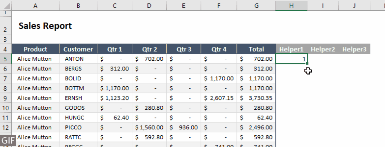
- No painel "Propriedades", vincule a caixa de texto a uma célula inserindo a referência da célula no campo "LinkedCell". Por exemplo, digitando "J2" garante que qualquer dado inserido na caixa de texto seja automaticamente atualizado na célula J2, e vice-versa.

- Clique em "Modo de Design" na aba "Desenvolvedor" para sair do "Modo de Design".


Agora, a caixa de texto permite que você insira texto.
Passo 2: Aplique a função FILTRAR
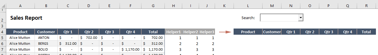
- Antes de usar a função FILTRAR, copie a linha de cabeçalho original para uma nova área. Aqui eu coloco a linha de cabeçalho abaixo da caixa de pesquisa.
Dica: Essa abordagem permite que os usuários vejam claramente os resultados sob os mesmos cabeçalhos de coluna dos dados originais.

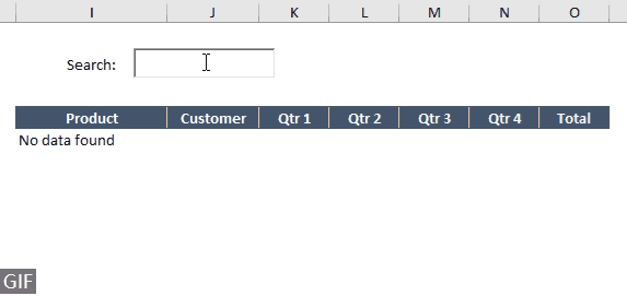
- Selecione a célula abaixo do primeiro cabeçalho (por exemplo, I5 neste exemplo), insira a seguinte fórmula nela e pressione a tecla "Enter" para obter o resultado.
=FILTER(Sheet2!$A$5:$G$281,Sheet2!$B$5:$B$281=J2,"No data found") Como mostrado na captura de tela acima, já que a caixa de texto agora não tem entrada, a fórmula exibe o resultado "Nenhum dado encontrado" em I5.


- Nesta fórmula:
- "Planilha2!$A$5:$G$281": $A$5:$G$281 é o intervalo de dados que você deseja filtrar na Planilha2.
- "Planilha2!$B$5:$B$281=J2": Esta parte define os critérios usados para filtrar o intervalo. Ele verifica cada célula na coluna B, da linha 5 à 281 na Planilha2, para ver se ela é igual ao valor na célula J2. J2 é a célula vinculada à caixa de pesquisa.
- "Nenhum dado encontrado": Se a função FILTRAR não encontrar nenhuma linha onde o valor na coluna B seja igual ao valor na célula J2, ela retornará "Nenhum dado encontrado".
- Esse método não diferencia maiúsculas de minúsculas, o que significa que ele corresponderá ao texto independentemente de você digitar em letras maiúsculas ou minúsculas.
Resultado: Teste a caixa de pesquisa
Agora vamos testar a caixa de pesquisa. Neste exemplo, quando eu insiro o nome de um cliente na caixa de pesquisa, os resultados correspondentes serão filtrados e exibidos imediatamente.

Crie uma caixa de pesquisa usando Formatação Condicional
A Formatação Condicional pode ser usada para destacar dados que correspondem a um termo de pesquisa, criando indiretamente um efeito de caixa de pesquisa. Esse método não filtra os dados, mas orienta visualmente você para as células relevantes. Esta seção mostrará como criar uma caixa de pesquisa usando Formatação Condicional no Excel.
Passo 1: Insira uma caixa de texto e configure as propriedades
- Vá para a aba "Desenvolvedor", clique em "Inserir" > "Caixa de Texto (Controle ActiveX)".
Dica: Se a aba "Desenvolvedor" não estiver visível na faixa de opções, você pode ativá-la seguindo as instruções deste tutorial: Como exibir/ativar a aba Desenvolvedor na Faixa de Opções do Excel?
- O cursor se transformará em uma cruz, e então você precisará arrastar o cursor para desenhar a caixa de texto no local da planilha onde deseja colocá-la. Após desenhar a caixa de texto, solte o mouse.
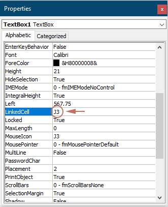
- Clique com o botão direito na caixa de texto e selecione Propriedades no menu de contexto.
- No painel "Propriedades", vincule a caixa de texto a uma célula inserindo a referência da célula no campo "LinkedCell". Por exemplo, digitando "J3" garante que qualquer dado inserido na caixa de texto seja automaticamente atualizado na célula J3, e vice-versa.
- Clique em "Modo de Design" na aba "Desenvolvedor" para sair do "Modo de Design".

Agora, a caixa de texto permite que você insira texto.
Passo 2: Aplique a Formatação Condicional para pesquisar dados
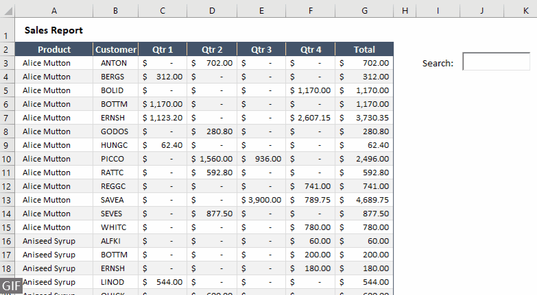
- Selecione todo o intervalo de dados a ser pesquisado. Aqui eu seleciono o intervalo A3:G279.
- Na aba "Página Inicial", clique em "Formatação Condicional" > "Nova Regra".
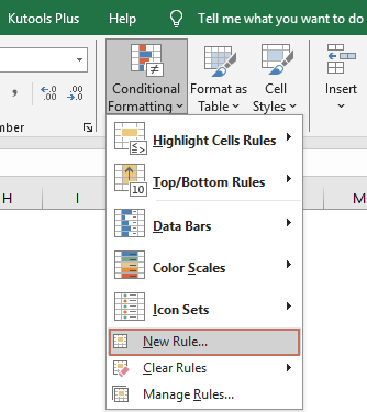
- Na caixa de diálogo "Nova Regra de Formatação":
- Selecione "Usar uma fórmula para determinar quais células formatar" nas opções de "Selecionar um Tipo de Regra".
- Insira a seguinte fórmula na caixa "Formatar valores onde esta fórmula for verdadeira".
=$B3=$J$3Aqui, "$B3" representa a primeira célula na coluna que você deseja comparar com os critérios de pesquisa no intervalo selecionado, e "$J$3" é a célula vinculada à caixa de pesquisa. - Clique no botão "Formatar" para especificar uma cor de preenchimento para os resultados da pesquisa.
- Clique no botão "OK". Veja a captura de tela:


Resultado
Agora vamos testar a caixa de pesquisa. Neste exemplo, quando eu insiro o nome de um cliente na caixa de pesquisa, as linhas correspondentes que contêm esse cliente na coluna B serão imediatamente destacadas com a cor de preenchimento especificada.
Crie uma caixa de pesquisa com combinações de fórmulas
Se você não está usando a versão mais recente do Excel e prefere não apenas destacar linhas, o método descrito nesta seção pode ser útil. Você pode usar uma combinação de fórmulas do Excel para criar uma caixa de pesquisa funcional em qualquer versão do Excel. Siga as etapas abaixo.
Passo 1: Crie uma lista de valores únicos a partir da coluna de pesquisa
- Neste caso, seleciono e copio o intervalo "B4:B281" para uma nova planilha.
- Depois de colar o intervalo em uma nova planilha, mantenha os dados colados selecionados, vá para a aba "Dados" e selecione "Remover Duplicatas".

- Na caixa de diálogo "Remover Duplicatas" que se abre, clique no botão "OK".
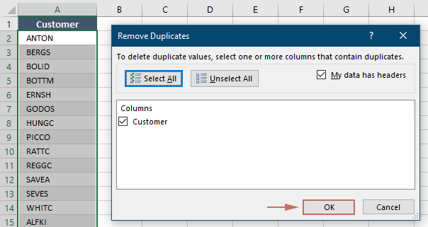
- Uma caixa de prompt do "Microsoft Excel" aparecerá para mostrar quantas duplicatas foram removidas. Clique em "OK".

- Após remover as duplicatas, selecione todos os valores únicos na lista, excluindo o cabeçalho, e atribua um nome a este intervalo inserindo-o na caixa "Nome". Aqui eu nomeei o intervalo como "Cliente".


Passo 2: Insira uma caixa de combinação e configure as propriedades
- Volte para a planilha que contém o conjunto de dados que você deseja pesquisar. Vá para a aba "Desenvolvedor", clique em "Inserir" > "Caixa de Combinação (Controle ActiveX)".
Dica: Se a aba "Desenvolvedor" não estiver visível na faixa de opções, você pode ativá-la seguindo as instruções deste tutorial: Como exibir/ativar a aba Desenvolvedor na Faixa de Opções do Excel?

- O cursor se transformará em uma cruz, e então você precisará arrastar o cursor para desenhar a caixa de combinação no local da planilha onde deseja colocar a caixa de pesquisa. Após desenhar a caixa de combinação, solte o mouse.
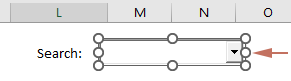
- Clique com o botão direito na caixa de combinação e selecione "Propriedades" no menu de contexto.

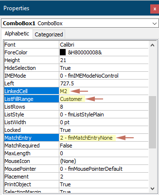
- No painel "Propriedades":
- Vincule a caixa de combinação a uma célula inserindo a referência da célula no campo "LinkedCell". Aqui eu digito "M2".
Dica: Especificar este campo garante que qualquer dado inserido na caixa de combinação será automaticamente atualizado na célula M2, e vice-versa.
- No campo "ListFillRange", insira o "nome do intervalo" que você especificou para a lista única na Etapa 1.
- Altere o campo "MatchEntry" para "2 – fmMatchEntryNone".
- Feche o painel "Propriedades".
- Vincule a caixa de combinação a uma célula inserindo a referência da célula no campo "LinkedCell". Aqui eu digito "M2".
- Clique em "Modo de Design" na aba "Desenvolvedor" para sair do Modo de Design.


Agora você pode selecionar qualquer item da caixa de combinação ou digitar o texto para pesquisar.
Passo 3: Aplique as fórmulas
- Crie três colunas auxiliares adjacentes ao intervalo de dados original. Veja a captura de tela:

- Na célula (H5) sob o título da primeira coluna auxiliar, insira a seguinte fórmula e pressione "Enter".
=ROWS($B$5:B5)Aqui "B5" é a célula que contém o nome do primeiro cliente da coluna a ser pesquisada.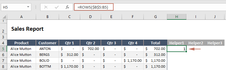
- Clique duas vezes no canto inferior direito da célula da fórmula, as células subsequentes serão automaticamente preenchidas com a mesma fórmula.
- Na célula (I5) sob o cabeçalho da segunda coluna auxiliar, insira a seguinte fórmula e pressione "Enter". Em seguida, clique duas vezes no canto inferior direito da célula da fórmula para preencher automaticamente as células abaixo com a mesma fórmula.
=IF(ISNUMBER(SEARCH($M$2,B5)),H5,"")Aqui "M2" é a célula vinculada à caixa de combinação.
- Na célula (J5) sob o cabeçalho da terceira coluna auxiliar, insira a seguinte fórmula e pressione "Enter". Em seguida, clique duas vezes no canto inferior direito da célula da fórmula para preencher automaticamente as células abaixo com a mesma fórmula.
=IFERROR(SMALL($I$5:$I$281,H5),"")
- Copie a linha de cabeçalho original para uma nova área. Aqui eu coloco a linha de cabeçalho abaixo da caixa de pesquisa.
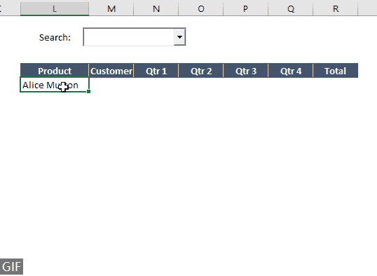
- Selecione a célula abaixo do primeiro cabeçalho (por exemplo, L5 neste exemplo), insira a seguinte fórmula nela e pressione a tecla "Enter".
=IFERROR(INDEX($A$5:$G$281,$J5,COLUMNS($L$4:L4)),"")Aqui "A5:G281" é todo o intervalo de dados que você deseja exibir na célula de resultado.
- Selecione esta célula de fórmula, arraste a "Alça de Preenchimento" para a direita e depois para baixo para aplicar a fórmula às colunas e linhas correspondentes.
 Notas:
- Como não há entrada na caixa de pesquisa, os resultados da fórmula mostrarão os dados brutos.
- Este método não diferencia maiúsculas de minúsculas, o que significa que ele corresponderá ao texto independentemente de você digitar em letras maiúsculas ou minúsculas.


Resultado
Agora vamos testar a caixa de pesquisa. Neste exemplo, quando eu insiro ou seleciono o nome de um cliente na caixa de combinação, as linhas correspondentes que contêm esse nome de cliente na coluna B serão filtradas e exibidas imediatamente no intervalo de resultados.

Criar uma caixa de pesquisa no Excel pode melhorar significativamente como você interage com seus dados, tornando suas planilhas mais dinâmicas e amigáveis. Seja optando pela simplicidade da função FILTRAR, pela assistência visual da Formatação Condicional ou pela versatilidade das combinações de fórmulas, cada método oferece ferramentas valiosas para aprimorar suas capacidades de manipulação de dados. Experimente essas técnicas para descobrir qual funciona melhor para suas necessidades e cenários de dados específicos. Para aqueles ansiosos para explorar mais as capacidades do Excel, nosso site conta com uma riqueza de tutoriais. Descubra mais dicas e truques do Excel aqui.
Melhores Ferramentas de Produtividade para Office
Impulsione suas habilidades no Excel com Kutools para Excel e experimente uma eficiência incomparável. Kutools para Excel oferece mais de300 recursos avançados para aumentar a produtividade e economizar tempo. Clique aqui para acessar o recurso que você mais precisa...
Office Tab traz interface com abas para o Office e facilita muito seu trabalho
- Habilite edição e leitura por abas no Word, Excel, PowerPoint, Publisher, Access, Visio e Project.
- Abra e crie múltiplos documentos em novas abas de uma mesma janela, em vez de em novas janelas.
- Aumente sua produtividade em50% e economize centenas de cliques todos os dias!
Todos os complementos Kutools. Um instalador
O pacote Kutools for Office reúne complementos para Excel, Word, Outlook & PowerPoint, além do Office Tab Pro, sendo ideal para equipes que trabalham em vários aplicativos do Office.
- Pacote tudo-em-um — complementos para Excel, Word, Outlook & PowerPoint + Office Tab Pro
- Um instalador, uma licença — configuração em minutos (pronto para MSI)
- Trabalhe melhor em conjunto — produtividade otimizada entre os aplicativos do Office
- Avaliação completa por30 dias — sem registro e sem cartão de crédito
- Melhor custo-benefício — economize comparado à compra individual de add-ins