Como somar com base em critérios de coluna e linha no Excel?
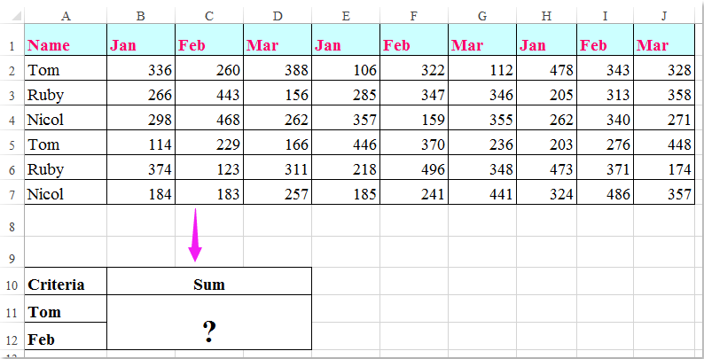
Tenho um intervalo de dados que contém cabeçalhos de linha e coluna, e agora quero fazer a soma das células que atendem aos critérios dos cabeçalhos de coluna e linha. Por exemplo, somar as células onde o critério da coluna é Tom e o critério da linha é Fev, conforme mostrado na captura de tela a seguir. Neste artigo, vou falar sobre algumas fórmulas úteis para resolver isso.
Somar células com base em critérios de coluna e linha usando fórmulas
 Somar células com base em critérios de coluna e linha usando fórmulas
Aqui, você pode aplicar as seguintes fórmulas para somar as células com base nos critérios de coluna e linha, faça o seguinte:
Insira qualquer uma das fórmulas abaixo em uma célula em branco onde deseja exibir o resultado:
=SOMARPRODUTO((A2:A7="Tom")*(B1:J1="Fev")*(B2:J7))
=SOMA(SE(B1:J1="Fev";SE(A2:A7="Tom";B2:J7)))
E então pressione as teclas Shift + Ctrl + Enter juntas para obter o resultado, veja a captura de tela:
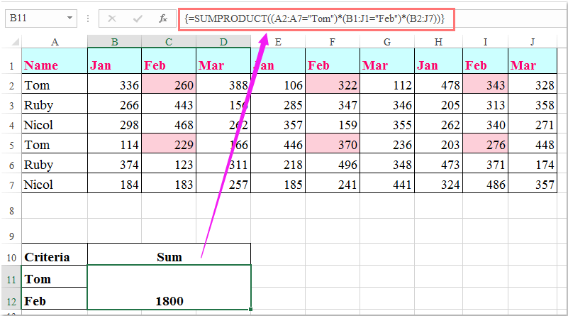
Observação: Nas fórmulas acima: Tom e Fev são os critérios de coluna e linha com base nos quais A2:A7, B1:J1 são os cabeçalhos de coluna e linha que contêm os critérios, e B2:J7 é o intervalo de dados que você deseja somar.

Desbloqueie a Magia do Excel com o Kutools AI
- Execução Inteligente: Realize operações de células, analise dados e crie gráficos — tudo impulsionado por comandos simples.
- Fórmulas Personalizadas: Gere fórmulas sob medida para otimizar seus fluxos de trabalho.
- Codificação VBA: Escreva e implemente código VBA sem esforço.
- Interpretação de Fórmulas: Compreenda fórmulas complexas com facilidade.
- Tradução de Texto: Supere barreiras linguísticas dentro de suas planilhas.
Melhores Ferramentas de Produtividade para Office
Impulsione suas habilidades no Excel com Kutools para Excel e experimente uma eficiência incomparável. Kutools para Excel oferece mais de300 recursos avançados para aumentar a produtividade e economizar tempo. Clique aqui para acessar o recurso que você mais precisa...
Office Tab traz interface com abas para o Office e facilita muito seu trabalho
- Habilite edição e leitura por abas no Word, Excel, PowerPoint, Publisher, Access, Visio e Project.
- Abra e crie múltiplos documentos em novas abas de uma mesma janela, em vez de em novas janelas.
- Aumente sua produtividade em50% e economize centenas de cliques todos os dias!
Todos os complementos Kutools. Um instalador
O pacote Kutools for Office reúne complementos para Excel, Word, Outlook & PowerPoint, além do Office Tab Pro, sendo ideal para equipes que trabalham em vários aplicativos do Office.
- Pacote tudo-em-um — complementos para Excel, Word, Outlook & PowerPoint + Office Tab Pro
- Um instalador, uma licença — configuração em minutos (pronto para MSI)
- Trabalhe melhor em conjunto — produtividade otimizada entre os aplicativos do Office
- Avaliação completa por30 dias — sem registro e sem cartão de crédito
- Melhor custo-benefício — economize comparado à compra individual de add-ins