Como mostrar o primeiro item na lista suspensa em vez de um espaço em branco?
As listas suspensas em planilhas do Excel são uma funcionalidade prática para agilizar e padronizar a entrada de dados — os usuários podem simplesmente selecionar entre opções predefinidas, em vez de digitar valores individualmente. No entanto, às vezes você pode encontrar uma situação em que, ao clicar em uma célula com lista suspensa, a seleção inicial aparece como um espaço em branco em vez do primeiro item de dados real. Esse problema geralmente ocorre se a lista de dados-fonte foi editada e linhas em branco permanecem no final, ou se itens próximos ao final foram excluídos, levando a validação de dados a incluir espaços vazios indesejados no início da lista. Especialmente com listas longas, ter que rolar constantemente além de entradas em branco até o primeiro item válido pode ser ineficiente e frustrante.

Resolver isso não apenas melhora a conveniência para os usuários, mas também ajuda a evitar a seleção acidental de valores em branco, o que poderia impactar tarefas subsequentes de processamento ou relatórios de dados. Neste artigo, você aprenderá métodos práticos para garantir que a primeira entrada na sua lista suspensa sempre apareça no topo, eliminando esses espaços em branco desnecessários.
Usando uma Tabela do Excel como Fonte de Dados
Mostrar o primeiro item na lista suspensa em vez de um espaço em branco com a função Validação de Dados
Uma maneira eficaz de evitar entradas em branco no início da sua lista suspensa é configurar sua Validação de Dados usando uma fórmula que determina dinamicamente o intervalo correto. Essa abordagem garante que apenas as células preenchidas da sua lista-fonte sejam incluídas, independentemente de quaisquer linhas vazias causadas pela exclusão de dados no final. Esta solução é especialmente adequada para usuários que frequentemente modificam a lista-fonte ou que desejam um ajuste baseado em fórmulas direto, sem precisar usar macros.
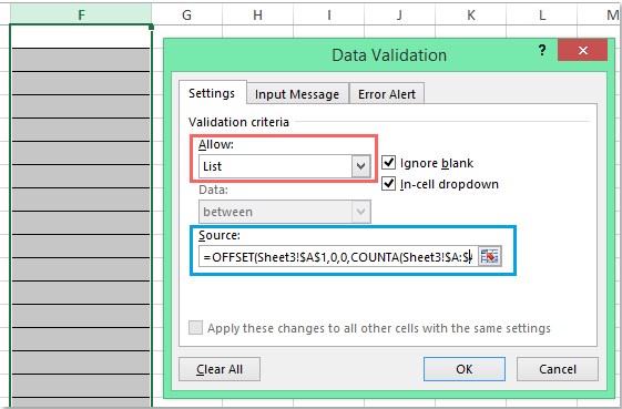
1. Selecione as células nas quais deseja criar a lista suspensa. Em seguida, vá para a faixa de opções do Excel e clique em Dados > Validação de Dados > Validação de Dados. A caixa de diálogo Validação de Dados será aberta, conforme mostrado abaixo:

2. Na guia Configurações na caixa de diálogo Validação de Dados, defina Permitir para Lista. Na caixa Origem, insira esta fórmula para referenciar dinamicamente apenas o intervalo contendo dados reais:
=OFFSET(Planilha3!$A$1,0,0,CONTARA(Planilha3!$A:$A)-1,1)
Nota: Nesta fórmula, Planilha3 refere-se à planilha onde seus dados-fonte residem, e A1 é a célula inicial da sua lista. Ajuste-os conforme necessário para o layout específico da sua planilha. O uso de CONTARA garante que apenas células não vazias sejam incluídas, começando em A1. Se sua lista-fonte contiver linhas em branco deliberadas dentro dela (não apenas no final), este método pode não excluir totalmente essas, então mantenha sua lista-fonte contígua para melhores resultados.
3. Clique em OK para aplicar as configurações. Agora, quando você clicar em qualquer uma das células da lista suspensa que configurou, a lista será exibida com o primeiro item de dados real no topo. Isso permanece verdadeiro mesmo se os dados-fonte mudarem, desde que o intervalo cubra todos os itens na coluna A e você não tenha células em branco dentro do bloco principal de dados. Veja o resultado abaixo:

Dica: Se mais tarde você precisar expandir ou reduzir sua lista-fonte, não precisa atualizar suas configurações de validação de dados. A fórmula se ajustará automaticamente, desde que não haja células em branco no início do intervalo. No entanto, esteja ciente de que, se houver um espaço em branco dentro da lista (não apenas no final), ele será ignorado na contagem de cálculo, mas poderá criar lacunas indesejadas na lista suspensa.
Problema potencial: Se sua fonte de dados puder conter lacunas intencionais, ou se você tiver células mescladas ou dados não contíguos, considere usar uma Tabela do Excel como seu intervalo-fonte, ou revise o método VBA abaixo para um tratamento mais flexível.
Mostrar automaticamente o primeiro item na lista suspensa em vez de um espaço em branco com código VBA
Em alguns cenários, ajustar apenas a origem da validação de dados não é suficiente — por exemplo, se seus dados mudam frequentemente, ou se há o risco de aparecerem espaços em branco por outras razões estruturais no intervalo-fonte. Com um código VBA simples, você pode garantir que sempre que uma célula com validação de dados for ativada, a lista suspensa selecione e exiba automaticamente o primeiro item disponível. Isso também pode aumentar a velocidade de entrada de dados, pois minimiza os cliques do usuário.
1. Depois de inserir sua lista suspensa, clique com o botão direito do mouse na guia da planilha que contém a lista suspensa e escolha Ver Código no menu de contexto. O editor Microsoft Visual Basic for Applications será exibido. Na janela, cole o seguinte código no módulo de planilha relevante (não em um módulo padrão). Esse código funcionará em segundo plano e redefinirá a lista suspensa cada vez que você selecionar uma célula de validação:
Código VBA: Mostrar automaticamente o primeiro item de dados na lista suspensa:
Private Sub Worksheet_SelectionChange(ByVal Target As Range)
'Updateby Extendoffice 20160725
    Dim xFormula As String
    On Error GoTo Out:
    xFormula = Target.Cells(1).Validation.Formula1
    If Left(xFormula, 1) = "=" Then
        Target.Cells(1) = Range(Mid(xFormula, 1)).Cells(1).Value
    End If
Out:
End Sub

2. Após colar o código, salve sua pasta de trabalho (de preferência como um arquivo habilitado para macro com extensão .xlsm) e feche a janela do editor VBA. Agora, retorne à sua planilha e tente clicar em qualquer célula com a lista suspensa — ao ativar a célula, a primeira entrada na sua lista suspensa será exibida automaticamente.
Dicas e considerações: Esta abordagem VBA é ideal quando você deseja uma experiência perfeita para os usuários, especialmente com listas-fonte dinâmicas ou longas, ou listas que podem conter entradas em branco inevitáveis. Lembre-se de habilitar macros para que isso funcione e informe outros usuários da pasta de trabalho, já que alguns ambientes restringem o uso de macros por razões de segurança.
Solução de problemas: Se o código não parecer funcionar, verifique novamente se ele está colocado na janela de código da planilha correta no editor VBA. Certifique-se também de que a lista suspensa usa uma lista padrão de Validação de Dados.
Limitação: A solução VBA só será acionada se o usuário selecionar a célula da lista suspensa; ela não funciona se a célula for preenchida por outros meios (como resultados de fórmulas ou via colagem). Se você remover a lista suspensa da célula ou mover a célula para outra planilha sem o código VBA, perderá o comportamento de seleção automática.
Usando uma Tabela do Excel como Fonte de Dados
Se sua lista-fonte da lista suspensa for dinâmica e você desejar maior facilidade de manutenção, considere converter sua lista-fonte em uma Tabela do Excel. As tabelas ajustam automaticamente seu tamanho à medida que os dados são adicionados ou removidos, então sua lista permanece atualizada. No entanto, observe que uma Tabela do Excel não exclui automaticamente células em branco — quaisquer entradas em branco na tabela ainda aparecerão na lista suspensa, a menos que você as filtre explicitamente (por exemplo, usando a função FILTRAR disponível no Excel 365 e Excel 2021).
1. Selecione seus dados-fonte e pressione Ctrl + T para convertê-los em uma Tabela. Certifique-se de que não há espaços em branco no início. Atribua um nome significativo à Tabela, como MinhaLista (usando a guia Design da Tabela).
2. Ao configurar a validação de dados, use a referência estruturada para a coluna da sua tabela. Na Origem da Validação de Dados, digite:
=INDIRECT("MyList[Column1]")Substitua Coluna1 pelo nome real da sua coluna (o cabeçalho da coluna). Este método inclui dinamicamente todos os itens na coluna da tabela que estão preenchidos, mantendo a integridade da lista à medida que você atualiza os dados.
Essa abordagem é especialmente adequada para ambientes onde os dados-fonte são atualizados regularmente e vários usuários precisam gerenciar a lista validada de forma eficiente.
Melhores Ferramentas de Produtividade para Office
Impulsione suas habilidades no Excel com Kutools para Excel e experimente uma eficiência incomparável. Kutools para Excel oferece mais de300 recursos avançados para aumentar a produtividade e economizar tempo. Clique aqui para acessar o recurso que você mais precisa...
Office Tab traz interface com abas para o Office e facilita muito seu trabalho
- Habilite edição e leitura por abas no Word, Excel, PowerPoint, Publisher, Access, Visio e Project.
- Abra e crie múltiplos documentos em novas abas de uma mesma janela, em vez de em novas janelas.
- Aumente sua produtividade em50% e economize centenas de cliques todos os dias!
Todos os complementos Kutools. Um instalador
O pacote Kutools for Office reúne complementos para Excel, Word, Outlook & PowerPoint, além do Office Tab Pro, sendo ideal para equipes que trabalham em vários aplicativos do Office.
- Pacote tudo-em-um — complementos para Excel, Word, Outlook & PowerPoint + Office Tab Pro
- Um instalador, uma licença — configuração em minutos (pronto para MSI)
- Trabalhe melhor em conjunto — produtividade otimizada entre os aplicativos do Office
- Avaliação completa por30 dias — sem registro e sem cartão de crédito
- Melhor custo-benefício — economize comparado à compra individual de add-ins