Como alterar a cor da forma com base no valor da célula no Excel?
Alterar a cor da forma com base em um valor específico de célula pode ser uma tarefa interessante no Excel. Por exemplo, se o valor da célula em A1 for menor que 100, a cor da forma será vermelha; se A1 for maior que 100 e menor que 200, a cor da forma será amarela; e quando A1 for maior que 200, a cor da forma será verde, conforme mostrado na captura de tela a seguir. Para alterar a cor da forma com base no valor de uma célula, este artigo apresentará um método para você.

Alterar a cor da forma com base no valor da célula com código VBA
Alterar a cor da forma com base no valor da célula com código VBA
O código VBA abaixo pode ajudá-lo a alterar a cor da forma com base no valor de uma célula. Por favor, siga os passos abaixo:
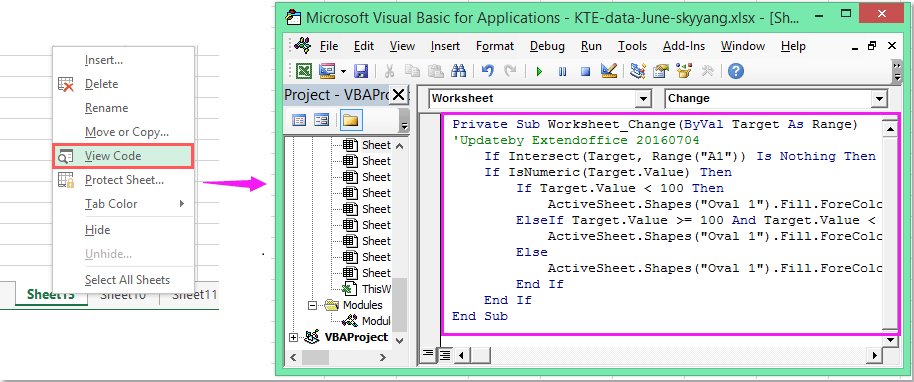
1. Clique com o botão direito do mouse na guia da planilha onde deseja alterar a cor da forma e, em seguida, selecione Visualizar Código no menu de contexto. Na janela Microsoft Visual Basic for Applications que apareceu, copie e cole o seguinte código na janela Módulo em branco.
Código VBA: Alterar a cor da forma com base no valor da célula:
Private Sub Worksheet_Change(ByVal Target As Range)
'Updateby Extendoffice 20160704
    If Intersect(Target, Range("A1")) Is Nothing Then Exit Sub
    If IsNumeric(Target.Value) Then
        If Target.Value < 100 Then
            ActiveSheet.Shapes("Oval 1").Fill.ForeColor.RGB = vbRed
        ElseIf Target.Value >= 100 And Target.Value < 200 Then
            ActiveSheet.Shapes("Oval 1").Fill.ForeColor.RGB = vbYellow
        Else
            ActiveSheet.Shapes("Oval 1").Fill.ForeColor.RGB = vbGreen
        End If
    End If
End Sub
2. E então, quando você inserir o valor na célula A1, a cor da forma será alterada de acordo com o valor da célula que você definiu.
Observação: No código acima, A1 é o valor da célula com base no qual a cor da forma será alterada, e Oval 1 é o nome da forma inserida. Você pode alterá-los conforme necessário.
Melhores Ferramentas de Produtividade para Office
Impulsione suas habilidades no Excel com Kutools para Excel e experimente uma eficiência incomparável. Kutools para Excel oferece mais de300 recursos avançados para aumentar a produtividade e economizar tempo. Clique aqui para acessar o recurso que você mais precisa...
Office Tab traz interface com abas para o Office e facilita muito seu trabalho
- Habilite edição e leitura por abas no Word, Excel, PowerPoint, Publisher, Access, Visio e Project.
- Abra e crie múltiplos documentos em novas abas de uma mesma janela, em vez de em novas janelas.
- Aumente sua produtividade em50% e economize centenas de cliques todos os dias!
Todos os complementos Kutools. Um instalador
O pacote Kutools for Office reúne complementos para Excel, Word, Outlook & PowerPoint, além do Office Tab Pro, sendo ideal para equipes que trabalham em vários aplicativos do Office.
- Pacote tudo-em-um — complementos para Excel, Word, Outlook & PowerPoint + Office Tab Pro
- Um instalador, uma licença — configuração em minutos (pronto para MSI)
- Trabalhe melhor em conjunto — produtividade otimizada entre os aplicativos do Office
- Avaliação completa por30 dias — sem registro e sem cartão de crédito
- Melhor custo-benefício — economize comparado à compra individual de add-ins