Como concatenar células se o mesmo valor existir em outra coluna no Excel?
Como mostrado na captura de tela abaixo, se você deseja concatenar células na segunda coluna com base nos mesmos valores na primeira coluna, há vários métodos que você pode usar. Neste artigo, apresentaremos três maneiras de realizar essa tarefa.

Concatenar células com o mesmo valor usando fórmulas e filtro
As seguintes fórmulas ajudam a concatenar as células correspondentes em uma coluna com base nos valores correspondentes em outra coluna.
1. Selecione uma célula em branco ao lado da segunda coluna (aqui selecionamos a célula C2), insira a fórmula =SE(A2<>A1;B2;C1 & "," & B2) na barra de fórmulas e pressione a tecla Enter.

2. Em seguida, selecione a célula C2 e arraste a Alça de Preenchimento para baixo até as células que você precisa concatenar.

3. Insira a fórmula =SE(A2<>A3;CONCATENAR(A2;",""";C2;""");"") na célula D2 e arraste a Alça de Preenchimento para baixo nas células restantes.

4. Selecione a célula D1 e clique em Dados > Filtro. Veja a captura de tela:

5. Clique na seta suspensa na célula D1, desmarque a caixa (Em branco) e clique no botão OK.

Você pode ver que as células são concatenadas se os valores da primeira coluna forem iguais.

Observação: Para usar as fórmulas acima com sucesso, os mesmos valores na coluna A devem ser contínuos.
Concatene células facilmente com o mesmo valor com o Kutools para Excel (vários cliques)
O método descrito acima requer a criação de duas colunas auxiliares e envolve várias etapas, o que pode ser inconveniente. Se você está procurando uma forma mais simples, considere usar a ferramenta Mesclar Linhas Avançado do Kutools para Excel. Com apenas alguns cliques, esta utilidade permite concatenar células usando um delimitador específico, tornando o processo rápido e sem complicações.
1. Clique em Kutools > Mesclar e Dividir > Mesclar Linhas Avançado para habilitar esse recurso.
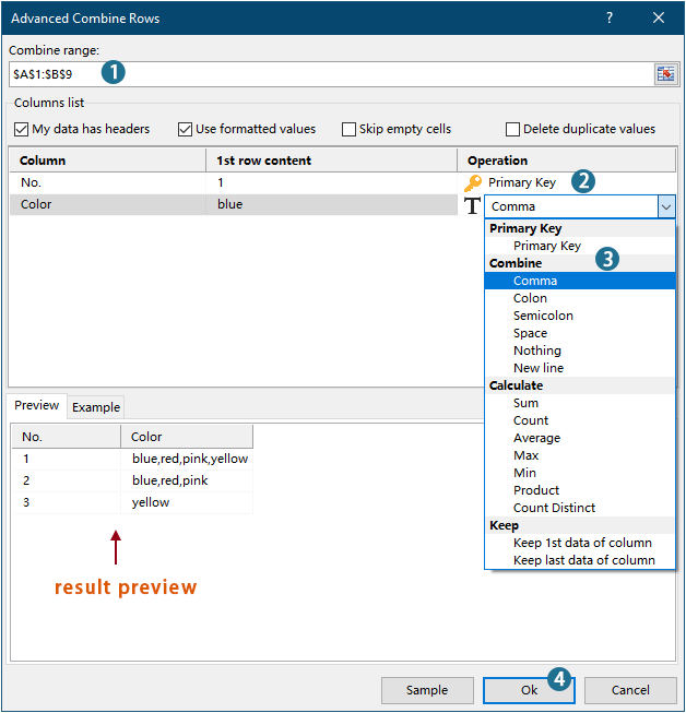
2. Na caixa de diálogo Mesclar Linhas Avançado, você só precisa:
- Selecionar o intervalo que deseja concatenar;
- Definir a coluna com os mesmos valores como a Coluna Chave.
- Especificar um separador para combinar as células.
- Clique em OK.
Resultado

Kutools para Excel - Potencialize o Excel com mais de 300 ferramentas essenciais. Aproveite recursos de IA permanentemente gratuitos! Obtenha Agora
- Para saber mais sobre este recurso, confira este artigo: Combine rapidamente valores iguais ou linhas duplicadas no Excel
Concatenar células com o mesmo valor usando código VBA
Você também pode usar o código VBA para concatenar células em uma coluna se o mesmo valor existir em outra coluna.
1. Pressione as teclas Alt + F11 para abrir a janela Microsoft Visual Basic Applications.
2. Na janela Microsoft Visual Basic Applications, clique em Inserir > Módulo. Em seguida, copie e cole o código abaixo na janela Módulo.
Código VBA: concatenar células com os mesmos valores
Sub ConcatenateCellsIfSameValues()
	Dim xCol As New Collection
	Dim xSrc As Variant
	Dim xRes() As Variant
	Dim I As Long
	Dim J As Long
	Dim xRg As Range
	xSrc    = Range("A1", Cells(Rows.Count, "A").End(xlUp)).Resize(, 2)
	Set xRg = Range("D1")
	On Error Resume Next
	For I = 2 To UBound(xSrc)
		xCol.Add xSrc(I, 1), TypeName(xSrc(I, 1)) & CStr(xSrc(I, 1))
	Next I
	On Error GoTo 0
	ReDim xRes(1 To xCol.Count + 1, 1 To 2)
	xRes(1, 1) = "No"
	xRes(1, 2) = "Combined Color"
	For I = 1 To xCol.Count
		xRes(I + 1, 1) = xCol(I)
		For J = 2 To UBound(xSrc)
			If xSrc(J, 1) = xRes(I + 1, 1) Then
				xRes(I + 1, 2) = xRes(I + 1, 2) & ", " & xSrc(J, 2)
			End If
		Next J
		xRes(I + 1, 2) = Mid(xRes(I + 1, 2), 2)
	Next I
	Set xRg = xRg.Resize(UBound(xRes, 1), UBound(xRes, 2))
	xRg.NumberFormat = "@"
	xRg = xRes
	xRg.EntireColumn.AutoFit
End SubObservações:
3. Pressione a tecla F5 para executar o código, então você obterá os resultados concatenados no intervalo especificado.

Demonstração: Concatene células facilmente com o mesmo valor com o Kutools para Excel
Melhores Ferramentas de Produtividade para Office
Impulsione suas habilidades no Excel com Kutools para Excel e experimente uma eficiência incomparável. Kutools para Excel oferece mais de300 recursos avançados para aumentar a produtividade e economizar tempo. Clique aqui para acessar o recurso que você mais precisa...
Office Tab traz interface com abas para o Office e facilita muito seu trabalho
- Habilite edição e leitura por abas no Word, Excel, PowerPoint, Publisher, Access, Visio e Project.
- Abra e crie múltiplos documentos em novas abas de uma mesma janela, em vez de em novas janelas.
- Aumente sua produtividade em50% e economize centenas de cliques todos os dias!
Todos os complementos Kutools. Um instalador
O pacote Kutools for Office reúne complementos para Excel, Word, Outlook & PowerPoint, além do Office Tab Pro, sendo ideal para equipes que trabalham em vários aplicativos do Office.
- Pacote tudo-em-um — complementos para Excel, Word, Outlook & PowerPoint + Office Tab Pro
- Um instalador, uma licença — configuração em minutos (pronto para MSI)
- Trabalhe melhor em conjunto — produtividade otimizada entre os aplicativos do Office
- Avaliação completa por30 dias — sem registro e sem cartão de crédito
- Melhor custo-benefício — economize comparado à compra individual de add-ins