Como encontrar a primeira ou última sexta-feira de cada mês no Excel?
Normalmente, a sexta-feira é o último dia útil do mês. Como você pode encontrar a primeira ou última sexta-feira com base em uma data específica no Excel? Neste artigo, vamos guiá-lo sobre como usar duas fórmulas para encontrar a primeira ou última sexta-feira de cada mês.
Encontre a primeira sexta-feira do mês
Encontre a última sexta-feira do mês
Encontre a primeira sexta-feira do mês
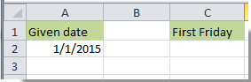
Por exemplo, há uma data fornecida 1/1/2015 localizada na célula A2, conforme mostrado na captura de tela abaixo. Se você deseja encontrar a primeira sexta-feira do mês com base na data fornecida, siga os passos abaixo.
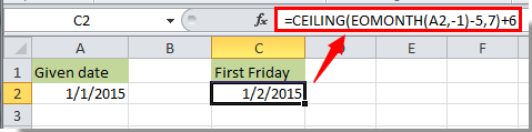
1. Selecione uma célula para exibir o resultado. Aqui selecionamos a célula C2.
2. Copie e cole a fórmula abaixo nela e pressione a tecla Enter.
=CEILING(EOMONTH(A2,-1)-5,7)+6
Observações:
Encontre a última sexta-feira do mês
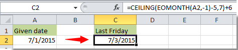
A data fornecida 1/1/2015 está localizada na célula A2. Para encontrar a última sexta-feira deste mês no Excel, siga os passos abaixo.
1. Selecione uma célula, copie a fórmula abaixo nela e pressione a tecla Enter para obter o resultado.
=DATE(YEAR(A2),MONTH(A2)+1,0)+MOD(-WEEKDAY(DATE(YEAR(A2),MONTH(A2)+1,0),2)-2,-7)

Observação: Você pode alterar A2 na fórmula para a célula de referência da sua data fornecida.
Artigos relacionados:
- Como encontrar os valores mais baixos e mais altos de 5 em uma lista no Excel?
- Como encontrar ou verificar se uma pasta de trabalho específica está aberta ou não no Excel?
- Como descobrir se uma célula está sendo referenciada em outra célula no Excel?
- Como encontrar a data mais próxima de hoje em uma lista no Excel?
Melhores Ferramentas de Produtividade para Office
Impulsione suas habilidades no Excel com Kutools para Excel e experimente uma eficiência incomparável. Kutools para Excel oferece mais de300 recursos avançados para aumentar a produtividade e economizar tempo. Clique aqui para acessar o recurso que você mais precisa...
Office Tab traz interface com abas para o Office e facilita muito seu trabalho
- Habilite edição e leitura por abas no Word, Excel, PowerPoint, Publisher, Access, Visio e Project.
- Abra e crie múltiplos documentos em novas abas de uma mesma janela, em vez de em novas janelas.
- Aumente sua produtividade em50% e economize centenas de cliques todos os dias!
Todos os complementos Kutools. Um instalador
O pacote Kutools for Office reúne complementos para Excel, Word, Outlook & PowerPoint, além do Office Tab Pro, sendo ideal para equipes que trabalham em vários aplicativos do Office.
- Pacote tudo-em-um — complementos para Excel, Word, Outlook & PowerPoint + Office Tab Pro
- Um instalador, uma licença — configuração em minutos (pronto para MSI)
- Trabalhe melhor em conjunto — produtividade otimizada entre os aplicativos do Office
- Avaliação completa por30 dias — sem registro e sem cartão de crédito
- Melhor custo-benefício — economize comparado à compra individual de add-ins