Como fazer a pesquisa VLOOKUP e retornar múltiplos valores correspondentes na horizontal no Excel?
VLOOKUP e retornar múltiplos valores na horizontal
 VLOOKUP e retornar múltiplos valores na horizontal
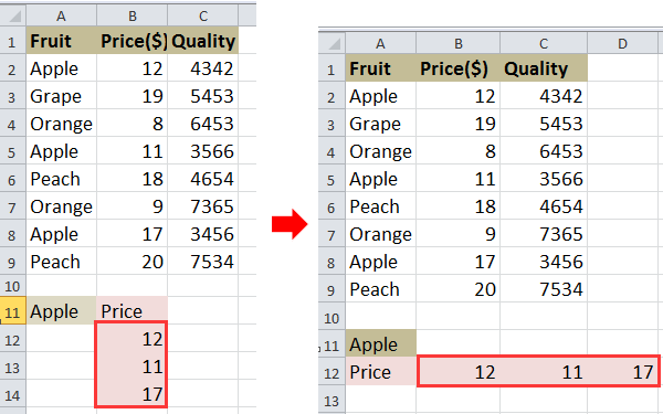
Por exemplo, você tem um intervalo de dados como mostrado na captura de tela abaixo, e deseja pesquisar os preços da Apple usando VLOOKUP.
1. Selecione uma célula e digite esta fórmula =INDEX($B$2:$B$9, SMALL(IF($A$11=$A$2:$A$9, ROW($A$2:$A$9)-ROW($A$2)+1), COLUMN(A1))) nela, e depois pressione Shift + Ctrl + Enter e arraste a alça de preenchimento automático para a direita para aplicar essa fórmula até que #NÚM! apareça. Veja a captura de tela:
2. Depois, exclua o #NÚM!. Veja a captura de tela:
Dica: Na fórmula acima, B2:B9 é o intervalo da coluna do qual você deseja retornar os valores, A2:A9 é o intervalo da coluna onde o valor de pesquisa está localizado, A11 é o valor de pesquisa, A1 é a primeira célula do seu intervalo de dados, A2 é a primeira célula do intervalo da coluna onde o valor de pesquisa está localizado.
Se você quiser retornar múltiplos valores verticalmente, pode ler este artigo Como pesquisar um valor e retornar múltiplos valores correspondentes no Excel?

Desbloqueie a Magia do Excel com o Kutools AI
- Execução Inteligente: Realize operações de células, analise dados e crie gráficos — tudo impulsionado por comandos simples.
- Fórmulas Personalizadas: Gere fórmulas sob medida para otimizar seus fluxos de trabalho.
- Codificação VBA: Escreva e implemente código VBA sem esforço.
- Interpretação de Fórmulas: Compreenda fórmulas complexas com facilidade.
- Tradução de Texto: Supere barreiras linguísticas dentro de suas planilhas.
Melhores Ferramentas de Produtividade para Office
Impulsione suas habilidades no Excel com Kutools para Excel e experimente uma eficiência incomparável. Kutools para Excel oferece mais de300 recursos avançados para aumentar a produtividade e economizar tempo. Clique aqui para acessar o recurso que você mais precisa...
Office Tab traz interface com abas para o Office e facilita muito seu trabalho
- Habilite edição e leitura por abas no Word, Excel, PowerPoint, Publisher, Access, Visio e Project.
- Abra e crie múltiplos documentos em novas abas de uma mesma janela, em vez de em novas janelas.
- Aumente sua produtividade em50% e economize centenas de cliques todos os dias!
Todos os complementos Kutools. Um instalador
O pacote Kutools for Office reúne complementos para Excel, Word, Outlook & PowerPoint, além do Office Tab Pro, sendo ideal para equipes que trabalham em vários aplicativos do Office.
- Pacote tudo-em-um — complementos para Excel, Word, Outlook & PowerPoint + Office Tab Pro
- Um instalador, uma licença — configuração em minutos (pronto para MSI)
- Trabalhe melhor em conjunto — produtividade otimizada entre os aplicativos do Office
- Avaliação completa por30 dias — sem registro e sem cartão de crédito
- Melhor custo-benefício — economize comparado à compra individual de add-ins