Como aplicar formatação condicional a datas menores ou maiores que hoje no Excel?
Gerenciar e acompanhar informações sensíveis ao tempo é crucial em muitas tarefas do Excel, desde o planejamento de projetos até as datas de vencimento de faturas ou o monitoramento de prazos. Uma necessidade frequente é distinguir visualmente datas que são anteriores ou posteriores à data atual. A formatação condicional do Excel permite destacar automaticamente essas datas, ajudando você a identificar rapidamente tarefas vencidas ou eventos futuros sem precisar rolar os dados manualmente. Neste tutorial, vamos apresentar várias abordagens práticas para destacar datas antes ou depois de hoje, incluindo ferramentas nativas do Excel e soluções avançadas com o Kutools para Excel. Você aprenderá a enfatizar eficientemente datas de vencimento, sinalizar atividades futuras e manter o controle em suas planilhas, independentemente do volume de dados ou das necessidades de atualização.
- Destacar datas anteriores a hoje ou datas futuras com Formatação Condicional
- Destacar datas anteriores a hoje ou datas futuras com Kutools AI
- Sinalizar e analisar datas com fórmulas de coluna auxiliar no Excel
Destacar datas anteriores a hoje ou datas futuras com Formatação Condicional
Suponha que você tenha uma coluna contendo várias datas, conforme ilustrado na captura de tela abaixo. Se você deseja destacar datas que já estão vencidas (anteriores a hoje) ou destacar datas futuras para ajudar no acompanhamento e planejamento, pode utilizar a formatação condicional do Excel com fórmulas baseadas na função HOJE. Esse recurso é especialmente valioso ao trabalhar com dados dinâmicos, pois a formatação será atualizada automaticamente todos os dias.

Primeiro, selecione sua lista de datas — para este exemplo, selecione as células A2:A15. Na guia Página Inicial, clique em Formatação Condicional > Gerenciar Regras. Consulte a captura de tela abaixo para orientação:

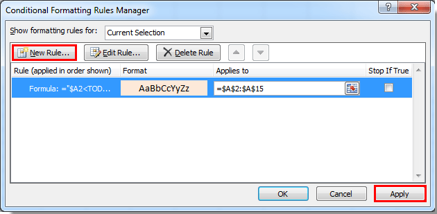
Assim que a caixa de diálogo Gerenciador de Regras de Formatação Condicional aparecer, clique no botão Nova Regra para criar uma regra personalizada baseada em fórmula.

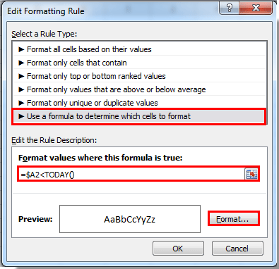
Na caixa de diálogo Nova Regra de Formatação:
• Escolha Usar uma fórmula para determinar quais células formatar. Essa opção permite um destaque flexível e baseado em datas.
• Para destacar datas anteriores a hoje, copie e cole a seguinte fórmula no campo Formatar valores onde esta fórmula for verdadeira:
=$A2<TODAY()• Para destacar datas que ocorrem após hoje (ou seja, datas futuras próximas), use esta fórmula:
=$A2>TODAY()• Em seguida, clique no botão Formatar para definir a aparência desejada (como alterar a cor de preenchimento ou o estilo da fonte). Veja o exemplo:
Especifique sua formatação desejada na caixa de diálogo Formatar Células (por exemplo, escolha uma cor para fazer com que as datas de vencimento ou datas futuras se destaquem), depois clique em OK.
De volta ao Gerenciador de Regras de Formatação Condicional, você verá sua nova regra listada. Para ativar a regra, clique em Aplicar. Se você deseja configurar o destaque tanto para datas de vencimento quanto para datas futuras, repita os passos para adicionar uma segunda regra usando a outra fórmula. Quando retornar ao Gerenciador de Regras, ambas as regras agora estarão visíveis.
Depois de confirmar com OK, sua planilha do Excel agora distinguirá visualmente datas antes e depois de hoje, oferecendo indicadores claros para promover ação ou atenção. As marcações de datas vencidas e futuras serão atualizadas automaticamente à medida que os dias mudam, para que você sempre veja os itens mais relevantes à primeira vista.

Aqui está o resultado: datas anteriores ou posteriores a hoje agora estão destacadas de acordo com sua seleção de formato, simplificando a revisão e o acompanhamento.

Dicas e Precauções: Certifique-se de que suas células de data estejam formatadas como datas (não texto) para que as fórmulas funcionem corretamente. Se você encontrar resultados inesperados, verifique novamente o formato da data. Para conjuntos de dados muito grandes, a formatação condicional pode impactar o desempenho, então considere limitar o intervalo de formatação sempre que possível.
Destacar datas anteriores a hoje ou datas futuras com Kutools AI
Para usuários que buscam uma maneira mais simples e inteligente de destacar datas vencidas ou futuras, o Kutools AI para Excel simplifica o processo. Em vez de criar regras de formatação condicional manualmente, você pode instruir o Kutools AI diretamente em linguagem simples. Esse método é ideal se você precisa destacar datas regularmente, mas quer economizar tempo ou evitar a configuração de fórmulas, ou se trabalha em ambientes onde precisão e eficiência são fundamentais.
Para usar o Kutools AI para destacar datas com base em sua relação com hoje:
- Clique em "Kutools" > "Assistente de IA" para abrir o painel "Assistente de IA do Kutools", depois faça as seguintes operações:
- Selecione o intervalo de datas que deseja examinar.
- No painel Assistente de IA, digite um comando como:
— Para datas vencidas: Destaque as datas antes de hoje com a cor azul clara no intervalo selecionado
— Para datas futuras: Destaque as datas após hoje com a cor azul clara no intervalo selecionado - Pressione Enter ou clique em Enviar. O Kutools AI analisará sua solicitação. Quando o processamento estiver concluído, clique em Executar para aplicar a formatação automaticamente.
O Kutools AI interpreta automaticamente sua intenção, escolhendo as fórmulas e formatos apropriados, economizando seu tempo e minimizando erros de configuração manual. Essa abordagem é particularmente útil em pastas de trabalho dinâmicas, para usuários menos familiarizados com fórmulas ou para aqueles que gerenciam grandes listas de datas frequentemente atualizadas.
Cuidado: O Kutools AI requer conectividade com a internet e a instalação atualizada do Kutools para Excel.
Sinalizar e analisar datas com fórmulas de coluna auxiliar no Excel
Em muitos casos do mundo real, você pode querer mais do que apenas codificação por cores — por exemplo, filtrar, classificar ou contar registros com base em se as datas são anteriores ou posteriores a hoje. Usar colunas auxiliares com fórmulas do Excel permite sinalizar essas situações claramente e usar outros recursos do Excel (como filtros ou Tabelas Dinâmicas) para análises detalhadas.
Prós: Fácil de configurar, suporta classificação/filtragem, funciona em todas as versões do Excel sem permissões especiais. Contras: Requer espaço adicional para colunas auxiliares; não fornece coloração direta, a menos que combinado com formatação condicional.
Aqui está como usar uma coluna auxiliar para análise rápida de datas:
1. Insira uma nova coluna ao lado da sua lista de datas (por exemplo, coluna B ao lado de suas datas em A2:A15).
2. Na célula B2 (assumindo que A2 é sua primeira data), insira esta fórmula para sinalizar datas vencidas:
=A2<TODAY()Essa fórmula retornará VERDADEIRO se a data em A2 for anterior a hoje e FALSO caso contrário.
3. Alternativamente, para destacar datas futuras, use:
=A2>TODAY()4. Pressione Enter para confirmar a fórmula, depois arraste a alça para baixo para preencher a coluna em todas as linhas contendo datas. Os resultados VERDADEIRO/FALSO agora podem ser usados para classificar ou filtrar registros por status vencido ou futuro.
Se você preferir rótulos de texto claros, substitua VERDADEIRO/FALSO por marcadores mais descritivos. Por exemplo:
=IF(A2<TODAY(),"Overdue",IF(A2>TODAY(),"Upcoming","Today"))Copie essa fórmula para todas as linhas relevantes conforme necessário. Você pode filtrar, classificar ou usar a coluna como critério em outros recursos do Excel, como Formatação Condicional ou Tabelas Dinâmicas. Essa abordagem é especialmente útil para relatórios, dashboards ou preparar documentos para impressão.
Nota: Se sua coluna de datas não for a coluna A, atualize a célula referenciada na fórmula de acordo. Certifique-se de que o tipo de dado para as células de data esteja definido como data, não texto, para evitar resultados inconsistentes.
Artigos relacionados:
- Como aplicar formatação condicional com base na primeira letra/caractere no Excel?
- Como aplicar formatação condicional se contiver #N/A no Excel?
- Como aplicar formatação condicional ou destacar a primeira recorrência no Excel?
- Como aplicar formatação condicional para destacar porcentagem negativa em vermelho no Excel?
Dicas rápidas de solução de problemas: Se o destaque ou as fórmulas não funcionarem como pretendido, sempre verifique sua formatação de data e os intervalos de fórmulas. Use o recurso Visualização na Formatação Condicional para inspecionar quais registros são afetados e verifique novamente se há regras duplicadas que podem se sobrepor ou contradizer. Para tabelas maiores, colunas auxiliares ou macros VBA podem simplificar a manutenção e economizar tempo quando atualizações frequentes forem necessárias. Explore vários métodos para encontrar o fluxo de trabalho mais adequado para seus cenários.
Melhores Ferramentas de Produtividade para Office
Impulsione suas habilidades no Excel com Kutools para Excel e experimente uma eficiência incomparável. Kutools para Excel oferece mais de300 recursos avançados para aumentar a produtividade e economizar tempo. Clique aqui para acessar o recurso que você mais precisa...
Office Tab traz interface com abas para o Office e facilita muito seu trabalho
- Habilite edição e leitura por abas no Word, Excel, PowerPoint, Publisher, Access, Visio e Project.
- Abra e crie múltiplos documentos em novas abas de uma mesma janela, em vez de em novas janelas.
- Aumente sua produtividade em50% e economize centenas de cliques todos os dias!
Todos os complementos Kutools. Um instalador
O pacote Kutools for Office reúne complementos para Excel, Word, Outlook & PowerPoint, além do Office Tab Pro, sendo ideal para equipes que trabalham em vários aplicativos do Office.
- Pacote tudo-em-um — complementos para Excel, Word, Outlook & PowerPoint + Office Tab Pro
- Um instalador, uma licença — configuração em minutos (pronto para MSI)
- Trabalhe melhor em conjunto — produtividade otimizada entre os aplicativos do Office
- Avaliação completa por30 dias — sem registro e sem cartão de crédito
- Melhor custo-benefício — economize comparado à compra individual de add-ins